A data analyst wanted to estimate the correlation between two variables, but he was concerned about the influence of a confounding variable that is correlated with them. The correlation might affect the apparent relationship between main two variables in the study. A common confounding variable is age because young people and older people tend to have different attitudes, behaviors, resources, and health issues.

This article gives a brief overview of partial correlation, which is a way to adjust or "control" for the effect of other variables in a study.

In this article, a confounding variable is a variable that is measured in the study and therefore can be incorporated into a model. This is different than a lurking variable, which is a variable that is not measured in the study. These definitions are common, but not universally used. The process of incorporating a confounding variable into a statistical model is called controlling for the variable.

Age as a confounding variable

Age is the classic confounding variable, so let's use a small SAS data set that gives the heights, weights, and ages of 19 school-age children. To make the analysis more general, I define macro variables Y1 and Y2 for the names of the two variables for which we want to find the correlation. For these data, the main variables are Y1=Height and Y2=Weight, and the confounding variable is Age.

To begin, let's compute the correlation between Y1 and Y2 without controlling for any other variables:

%let DSName = sashelp.Class;
%let Y1 = Height;
%let Y2 = Weight;
 
proc corr data=&DSName noprob plots(maxpoints=none)=scatter(ellipse=none);
   var &Y1;
   with &Y2;
run;

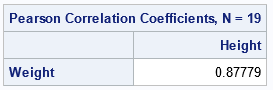
The output from the procedure indicates that Y1 and Y2 are strongly correlated, with a correlation of 0.88. But the researcher suspects that the ages of the students are contributing to the strong association between height and weight. You can test this idea graphically by creating a scatter plot of the data and coloring the markers according to the value of a third variable, as follows.

%let ControlVars = Age;         /* list one or more control variables */
 
title "Color Markers by a Confounding Variable";
proc sgplot data=&DSName;
   scatter x=&Y1 y=&Y2 / colorresponse=%scan(&ControlVars, 1)   /* color by first control var */
                         markerattrs=(symbol=CircleFilled size=14) FilledOutlinedMarkers
                         colormodel=TwoColorRamp;
run;

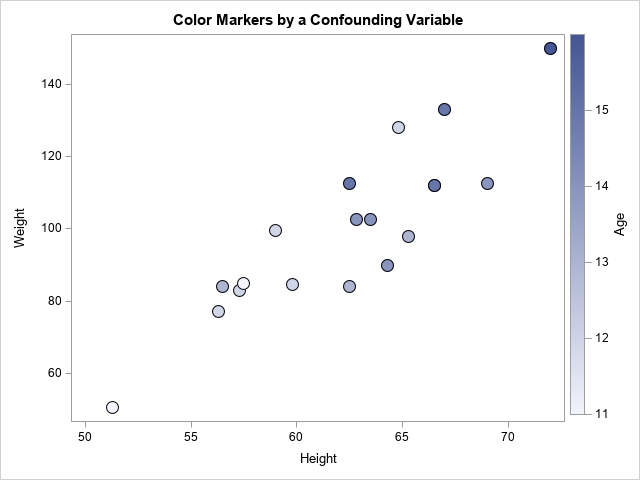
The graph shows that low values of height and weight are generally associated with low values of age, which are light blue in color. Similarly, high values of height and weight are generally associated with high values of age, which are colored dark blue. This indicates that the age variable might be affecting the correlation, or even might be responsible for it. One way to "adjust" for the age variable is to use partial correlation.

What is partial correlation?

A partial correlation is a way to adjust a statistic to account for one or more additional covariates. The partial correlation between variables Y1 and Y2 while adjusting for the covariates X1, X2, X3, ... is computed as follows:

1. Regress Y1 onto the covariates and calculate the residuals for the model. Let R1 be the variable that contains the residuals for the model.
2. Regress Y2 onto the covariates. Let R2 be the column of residuals.
3. Compute the correlation between R1 and R2. This is the partial correlation between Y1 and Y2 after adjusting for the covariates.

How to compute partial correlation in SAS

SAS provides an easy way to compute the partial correlation. PROC CORR supports the PARTIAL statement. On the PARTIAL statement, you list the covariates that you want to account for. PROC CORR automatically computes the regression models and provides the correlation of the residuals. In addition to the partial Pearson correlation, PROC CORR can report the partial versions of Spearman's rank correlation, Kendall's association, and the partial variance and standard deviation. The partial mean is always 0, so it is not reported.

The following call to PROC CORR shows the syntax of the PARTIAL statement:

proc corr data=&DSName plots(maxpoints=none)=scatter(ellipse=none);
   var &Y1;
   with &Y2;
   partial &ControlVars; 
run;

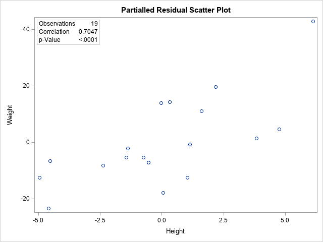
The output includes tables and a scatter plot of the residuals of Y2 versus the residuals of Y1. Only the graph is shown here. The graph includes an inset that tells you that the partial correlation is 0.7, which is less than the unadjusted correlation (0.88). Although the axes are labeled by using the original variable names, the quantities that are graphed are residuals from the two regressions. Notice that both axes are centered around zero, and the range of each axis is different from the original range.

How should you interpret this graph and the partial correlation statistic? The statistic tells you that after adjusting for age, the correlation between the heights and weights of students is about 0.7. The graph shows the scatter plot of the residual values of the heights and weights after regressing those variables onto the age variable.

How to manually calculate partial correlations

You can obtain the partial correlation manually by performing each step of the computation. This is not necessary in SAS, but it enables you to verify the computations that are performed by the PARTIAL statement in PROC CORR. To verify the output, you can manually perform the following steps:

1. Use PROC REG to regress Y1 onto the covariates. Use the OUTPUT statement to save the residuals for the model.
2. Use PROC REG to regress Y2 onto the covariates. Save the residuals for this model, too.
3. Merge the two output data sets.
4. Use PROC CORR to compute the (raw) correlation between the residual variables. This is the partial correlation between Y1 and Y2 after adjusting for the covariates.

The following SAS statements perform this analysis:

/* 1. Regress Y1 onto covariates and save residuals */
proc reg data=&DSName noprint;
   model &Y1 = &ControlVars;
   output out=RegOut1 R=Part_&Y1;
quit;
/* 2. Regress Y2 onto covariates and save residuals */
proc reg data=&DSName noprint;
   model &Y2 = &ControlVars;
   output out=RegOut2 R=Part_&Y2;
quit;
/* 3. Merge the two sets of residuals */
data RegOut;
merge RegOut1(keep=&ControlVars Part_&Y1)
      RegOut2(keep=Part_&Y2);
label Part_&Y1 = "Residual of &Y1 ~ (&ControlVars)"
      Part_&Y2 = "Residual of &Y2 ~ (&ControlVars)";
run;
/* 4. Display the correlation between the residuals */
proc corr data=RegOut plots=scatter(ellipse=none);
   var Part_&Y1;
   with Part_&Y2;
run;

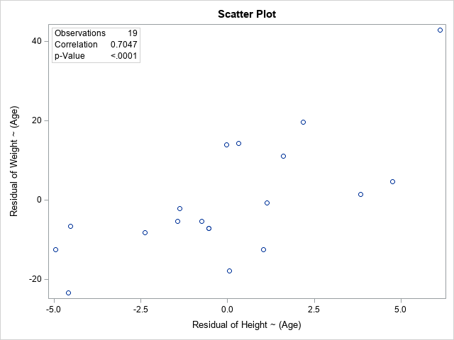
As expected, the graph of the residual values is the same graph that was created by using the PARTIAL statement. As expected, the inset shows that the correlation between the residuals is the same value that was reported by using the PARTIAL statement.

Summary

It can be useful to account for or "adjust" a statistic to account for other variables that might be strongly correlated with the main variables in the analysis. One way to adjust for confounding variables is to regress the main variables onto the confounding variables and look at the statistic for the residual values. This is called a "partial" statistic and is supported in SAS by using the PARTIAL statement in several procedures. This article shows how to use the PARTIAL statement in PROC CORR to compute the partial correlation. It also shows how to manually reproduce the computation by explicitly performing the regressions and calculating the correlation of the residuals.

Appendix: PROC REG also provides (squared) partial correlations

In SAS, there are often multiple ways to get the same statistic. It turns out that you can get the SQUARED Pearson partial correlation from PROC REG by using the PCORR2 option on the MODEL statement. I don't often use this option, but for completeness, the following statements compute the squared partial correlation between Y2 and Y1:

proc reg data=&DSName plots=none;
   model &Y2 = &Y1 &ControlVars / pcorr2;
   ods select ParameterEstimates;
quit;

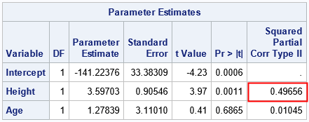
The "Type II Squared Partial Correlation" between Y2 and Y1 is 0.49656. If you take the square root of that number, you get ±0.7047. The tabular output from PROC REG does not enable you to determine whether the partial correlation is positive or negative.