A SAS programmer asked for help to simulate data from a distribution that has certain properties. The distribution must be supported on the interval [a, b] and have a specified mean, μ, where a < μ < b. It turns out that there are infinitely many distributions that satisfy these conditions. This article describes the shapes for a family of beta distributions that solve this problem.

Common bounded distributions

There are three common distributions that are used to model data on a bounded interval:

• The triangular distribution has a peak (mode) that is easy to specify. The PDF looks like a triangle, so this distribution might not be a good model for real data.
• The PERT distribution also has a mode that is easy to specify. The PERT distribution is a particular example of a beta distribution that is used in decision analysis.
• The two-parameter beta distribution is a flexible family that can model a wide range of distributional shapes.

An interesting fact about the two-parameter beta distribution is that you can model many different shapes. The parameters for the beta distribution enable you to model distributions for which the PDF is decreasing, increasing, U-shaped, and has either positive or negative skewness.

If Y is a beta-distributed random variable on [0,1] that has mean p, then X = (b – a)Y + a is a random variable on [a, b] that has mean μ = (b – a)p + a. Thus, we can simulate beta-distributed data, and then scale and translate the data to any other bounded interval.

Beta distributions that have a common mean

Let's examine the shapes of some beta distributions that all have the same mean, p, in [0,1]. The mean of the Beta(α, β) distribution is p = α/(α+β). Thus, for any specified mean, there is a one-parameter family of beta distributions, each with a different shape, that all have the same mean. For any value of the β parameter, choose α = p / (1 – p) β to ensure that the Beta(α, β) distribution has mean p.

Let's compute the PDF for a few members of the family to see what they look like. In the following program, I specify that I want a beta distribution that has mean value p = 2/3, which forces α = 2 β. I then plot the PDF for several values of β to visualize the different shapes:

/* show PDFs for a sample of (alpha, beta) values such that the
   Beta(alpha, beta) distribution has mean=2/3 */ 
data BetaPDF;
keep alpha beta y pdf;
p = 2/3;                     /* mean of Y ~ Beta(alpha, beta) distribution */
do beta = 0.2, 0.8, 2, 6;
   alpha = p/(1-p) * beta;   /* choose alpha so that distrib has mean p */
   do y = 0.01 to 0.99 by 0.01;
      PDF = pdf("beta", y, alpha, beta);
      output;
   end; 
end;
run;
 
title "A Family of Beta Distributions for Mean = 2/3";
proc sgplot data=BetaPDF;
   series x=y y=PDF / group=beta lineattrs=(thickness=2);
   yaxis min=0 max=4 label="Density";
run;

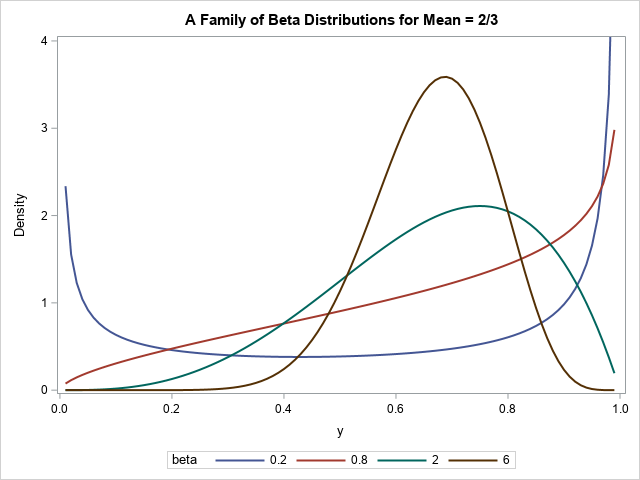
Notice the shapes of the resulting beta distributions:

• The PDF for β=0.2 is U-shaped.
• The PDF for β=0.8 is monotonic increasing.
• The PDF for β=2 has a mode at 0.75.
• The PDF for β=6 has a mode at 0.6875. It appears to be approximately bell-shaped.

All these distributions have the same mean, which is p = 2/3. As β increases, the distribution becomes nearly normal, and the mode approaches the mean.

Simulate data from a bounded distribution with a specified mean

The PDF of the distributions is easier to visualize than a random sample. But you can modify the program to generate random variates instead of a PDF. To obtain a random sample on [a, b] that has mean μ, you can transform the problem: use the beta distribution to simulate a sample on [0, 1], then transform the data into the interval [a, b].

For example, suppose you want a random sample from a distribution that has mean 20 and is bounded on the interval [10, 25]. Because 20 is two-thirds of the way between 10 and 25, you can simulate from a beta distribution on [0, 1] that has mean p = 2/3. If Y is a beta-distributed random variable on [0, 1], then X = (25-10)*Y + 10 is a random variable on [10, 25].

The following SAS DATA step demonstrates this technique. Because the problem does not have a unique solution, the program generates six random samples, each with N=200 observations. Each sample has a different shape, but they are all generated from a distribution whose mean is 20.

/* Define interval [a,b] and mean, mu */
%let a = 10;
%let b = 25;
%let mu = 20;                /* note that mu is 2/3 of the way from a to b */
/* if X is r.v. on [a,b] with mean mu, then 
   Y = (X-a)/(b-a) is r.v. on [0,1] with mean p=a + (b-a)*mu */
data BetaSim;
call streaminit(1234);
keep alpha beta x y;
a = &a; b = &b; mu = μ
p = (mu - a)/(b-a);          /* mean of Y ~ Beta in [0, 1] */
do beta = 0.2, 0.5, 0.8, 1, 2, 6;
   alpha = p/(1-p) * beta;   /* choose alpha so that distrib has mean p */
   do i = 1 to 200;                  /* N = 200 for this example */
      y = rand("beta", alpha, beta); /* Y ~ Beta(alpha, beta) on [0,1] */
      x = (b-a)*y + a;               /* transform values into [a,b] */
      output;
   end; 
end;
run;
 
proc sgpanel data=BetaSim;
   panelby alpha beta / columns=3;
   histogram x;
   colaxis grid;
run;

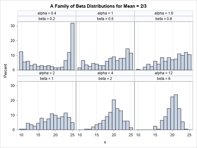
The panel shows six different samples. Each sample is drawn from a distribution that has mean 20. Four of the samples are generated from a (rescaled) distribution that was shown in the previous section. As you can see, the shape of the distributions vary. Some are U-shaped, some are nearly linear, and some are bell-shaped.

If you want a unique solution to this problem, you must add an additional constraint. A common choice is to match not just the mean of some sample data, but also the variance. These beta distributions all have different variances, so adding a constraint on the variance ensures a unique beta distribution.

Summary

This article shows how to simulate data from a distribution on the interval [a, b] that has a specified mean, μ. There are infinitely many distributions that satisfy these constraints. This article visualizes the shapes for a family of beta distributions that you can use to solve this problem. To get a unique solution, you can specify an additional requirement, such as a value for the variance.