Recently, I needed to write a program that can provide a solution to a regression-type problem, even when the data are degenerate. Mathematically, the problem is an overdetermined linear system of equations X*b = y, where X is an n x p design matrix and y is an n x 1 vector. For most data, you can obtain a least squares solution by solving the "normal equations" for b. In matrix notation, the normal equations are the matrix system (X`*X)*b = X`*y. However, if the columns of the design matrix are linearly dependent, the matrix (X`*X) is rank-deficient and the least squares system is singular. In the event of a singular system, I wanted to display a warning in the log.

A previous article shows that you can use a generalized inverse to construct a special solution for a rank-deficient system of equations. The special solution has the smallest L₂ norm among the infinitely many possible solutions. As I have previously discussed, one way to obtain a minimal-norm solution is to use the Moore-Penrose generalized inverse, which you can do by using the GINV function in SAS/IML software.

Unfortunately, the GINV function in SAS/IML does not indicate whether the input matrix is singular, which makes it difficult to display a warning in the log. However, there is a second option: the SAS/IML language supports the APPCORT subroutine, which returns the minimal-norm solution and an integer that specifies the number of linear dependencies among the columns of the design matrix. The integer is sometimes called the co-rank of the matrix. If the co-rank is 0, the matrix is full rank.

Least squares solutions and the number of linear dependencies

The following 7 x 5 design matrix contains five linearly independent columns. Therefore, the normal equations are nonsingular. You can obtain a least squares solution by using many methods. For nonsingular systems, I like to use the SOLVE function, but the following program also demonstrates that you can also use the GINV function or the APPCORT subroutine.

proc iml;
reset fuzz;  /* print tiny numbers as 0 */
X = {1 0 1 0 0,
     1 0 0 1 0,
     1 0 0 0 1,
     0 1 1 0 0,
     0 1 0 1 0,
     0 1 0 0 1,
     0 0 1 1 1};
y = { 3, 2, 4, 2, 1, 3, 3 };
 
/* find LS solution: min  |X*b-y|^2 by solving X`*x*b = X`*y for b */
A = X`*X;
z = X`*y;
 
b_Solve = solve(A, z); /* solve a nonsingular linear system */
 
Ainv = ginv(A);              /* find generalized inverse (uses SVD) */
b_Ginv = Ainv*z;
 
call appcort(b_Appcort, numLinDep, A, z); /* find LS soln (uses QR) */
print b_Solve b_Ginv b_Appcort, numLinDep;

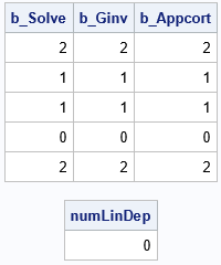
The output shows that all three methods give the same least squares solution for the nonsingular system. However, notice that the APPCORT subroutine provides more information. The subroutine returns the solution but also a scalar that indicates the number of linear dependencies that were detected while solving the system. For a nonsingular system, the number is zero. However, the next section repeats the analysis with a design matrix that has collinearities among the columns.

Least squares solutions when there are collinearities

If one of the columns of X is a linear combination of other columns, the SOLVE function will display an error message: ERROR: (execution) Matrix should be non-singular. In contrast, both the GINV function and the APPCORT routine can solve the resulting rank-deficient system of normal equations. In addition, the APPCORT subroutine provides information about whether the system was singular. If so, it tells you the number of collinearities.

The following program sets the fifth column of X to be a linear combination of two other columns. This causes the normal equations to be singular. Both the GINV function and the APPCORT subroutine solve the singular system by returning the solution that has the smallest 2-norm. The APPCORT subroutine also provides an integer that tells you the number of linear dependencies among the columns of X:

/* change X matrix so that the 5th column is a linear 
   combination of the first and 4th columns */
X[,5] = X[,1] + X[,4];
 
A = X`*X;
z = X`*y;
 
Ainv = ginv(A);              /* find generalized inverse (uses SVD) */
b_Ginv = Ainv*z;
 
call appcort(b_Appcort, numLinDep, A, z); /* find LS soln (uses QR) */
print b_Ginv b_Appcort, numLinDep;

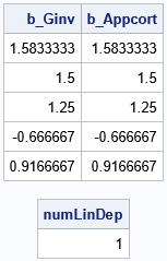
Notice that the GINV function and the APPCORT subroutine give the same solution (the one with minimal 2-norm). However, the APPCORT subroutine also tells you that the system is singular and that there is one linear dependency among the columns of X.

Summary

In summary, the APPCORT subroutine enables you to solve a least squares system, just like the SOLVE function and the GINV function. However, when the system is singular, the SOLVE function stops and displays an error. In contrast, the GINV function returns a solution. So does the APPCORT subroutine, and it also alerts you to the fact that the system is singular.

For the curious, the SOLVE function uses an LU decomposition to solve linear systems. The GINV function uses an SVD decomposition, and the APPCORT subroutine uses a QR decomposition. If you want to see the QR factorization that the APPCORT subroutine uses, you can use the COMPORT subroutine to get it.