Tukey's ladder of variable transformations

John Tukey was an influential statistician who proposed many statistical concepts. In the 1960s and 70s, he was fundamental in the discovery and exposition of robust statistical methods, and he was an ardent proponent of exploratory data analysis (EDA). In his 1977 book, Exploratory Data Analysis, he discussed a small family of power transformations that you can use to explore the relationship between two variables. Given bivariate data (x1, y1), (x2, y2), ..., (xn, yn), Tukey's transformations attempt to transform to the Y values so that the scatter plot of the transformed data is as linear as possible, and the relationship between the variables is simple to explain.

Tukey's Transformations

Tukey's transformations depend on a "power parameter," λ, which can be either positive or negative. When Y > 0, the transformations are as follows:

When λ > 0, the transformation is T(y; λ) = y^λ.
When λ = 0, the transformation is T(y; λ) = log(y).
When λ < 0, the transformation is T(y; λ) = –(y^λ).

If not all values of Y are positive, it is common to shift Y by adding a constant to every value. A common choice is to add c = 1 – min(Y) to every value. This ensures that the shifted values of Y are positive, and the minimum value is 1.

Although Tukey's transformation is defined for all values of the parameter, λ, he argues for using values that result in simple relationships such as integer powers (squares and cubes), logarithms, and reciprocal power laws such as inverse-square laws. Thus, he simplified the family to the following small set of useful transformations:

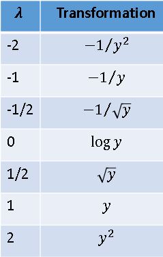
Some practitioners add -3, -1/3, 1/3, and 3 to this set of transformations. Tukey's ladder of transformation is similar to the famous Box-Cox family of transformations (1964), which I will describe in a subsequent article. The Box-Cox transformations have a different objective: they transform variables to acieve normality, rather than linearity.

A graphical method for Tukey's transformation

Tukey proposed many graphical techniques for exploratory data analysis. To explore whether a transformation of the Y variable results in a nearly linear relationship with the X variable, he suggests plotting the data. This is easily performed by using a SAS DATA step to transform the Y variable for each value of λ in the set {-2, -1, -1/2, 0, 1/2, 1, 2}. To ensure that the transformation only uses positive values, the following program adds c = 1 - min(Y) to each value of Y before transforming. The resulting scatter plots are displayed by using PROC SGPANEL.

/* define the data set and the X and Y variables */
%let dsName = Sashelp.Cars;
%let XName = Weight;
%let YName = MPG_Highway;
 
/* compute c = 1 - min(Y) and put in a macro variable */
proc sql noprint;                              
 select 1-min(&YName) into :c trimmed 
 from &dsName;
quit;
%put &=c;
 
data TukeyTransform;
array lambdaSeq[7] _temporary_ (-2, -1, -0.5, 0, 0.5, 1, 2);
set &dsName;
x = &XName;
y = &YName + &c;  /* offset by c to ensure Y >= 1 */
do i = 1 to dim(lambdaSeq);
   lambda = lambdaSeq[i];
   if lambda=0 then        z = log(y);
   else if lambda > 0 then z = y**lambda;
   else                    z = -(y**lambda);
   output;
end;
keep lambda x y z;
label x="&xName" y="&yName" z="Transformation of &YName";
run;
 
ods graphics / width=400px height=840px;
title "Tukey's Ladder of Transformations";
proc sgpanel data=TukeyTransform;
   panelby lambda / layout=rowlattice uniscale=column onepanel rowheaderpos=right;
   scatter x=x y=z;
   rowaxis grid; colaxis grid;
run;

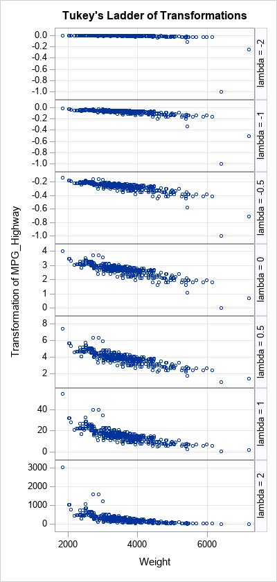
The panel of scatter plots shows seven transformations of the Y variable plotted against X. It is difficult to visually discern which plot is "most linear." The graph for λ=0 seems to be most linear, but the scatter plot for λ=0.5 also have very little curvature.

This panel of graphs is typical. Graphical methods can hint at the relationships between variables, but analytical techniques are often necessary to quantify the relationships. I put the name of the data set and the name of the variables in macro variables so that you can easily run the code on other data and investigate how it works on other examples.

An analytical method for Tukey's transformation

Tukey emphasized graphical methods in Exploratory Data Analysis (1977), but his ladder of transformations has a rigorous statistical formulation. The correlation coefficient is a measure of linearity in a scatter plot, so for each value of λ you can compute ρ_λ = corr(X, T(Y; λ)), where T(Y; λ) is the Tukey transformation for the parameter λ. The value of λ that results in the correlation that has the largest magnitude (closest to ±1) is the optimal parameter. In SAS, you can sort the transformed data by the Lambda variable and use PROC CORR to compute the correlation for each parameter value:

proc sort data=TukeyTransform;
   by lambda;
run;
 
/* compute corr(X, T(Y; lambda)) for each lambda */
proc corr data=TukeyTransform outp=CorrOut noprint;
   by lambda;
   var Z;
   with X;
run;
 
proc print data=CorrOut(where=(_TYPE_="CORR")) noobs label;   
   var lambda z;
   label z="corr(x, T(y))";
run;

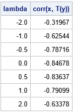
The correlation coefficients indicate that λ=0 results in a correlation of -0.85, which is the largest magnitude. For these data, λ=0.5 also does a good job of linearizing the data (ρ=-0.84). Several values of λ result in a correlation coefficient that is very strong, which is why it is difficult to find the best parameter by visually inspecting the graphs.

Summary

Tukey's ladder of transformations is a way to check whether two variables, X and Y, have a simple nonlinear relationship. For example, they might be related by a square-root or a logarithmic transformation. By using Tukey's ladder of transformations, you can discover relationships between variables such as inverse square laws, reciprocal laws, power laws, and logarithmic/exponential laws.

Blogs