I previously wrote about partial leverage plots for regression diagnostics and why they are useful. You can generate a partial leverage plot in SAS by using the PLOTS=PARTIALPLOT option in PROC REG. One useful property of partial leverage plots is the ability to graphically represent the null hypothesis that a regression coefficient is 0. John Sall ("Leverage Plots for General Linear Hypotheses", TAS, 1990) showed that you could add a confidence band to the partial regression plot such that if the line segment for Y=0 is not completely inside the band, then you reject the null hypothesis.

This article shows two ways to get the confidence band. The easy way is to write the partial leverage data to a SAS data set and use the REG statement in PROC SGPLOT to overlay a regression fit and a confidence band for the mean. This way is easy to execute, but it requires performing an additional regression analysis for every effect in the model. A second way (which is due to Sall, 1990) computes the confidence band directly from the statistics on the original data. This article shows how to use the SAS/IML language to compute the confidence limits from the output of PROC REG.

Confidence limits on a partial leverage plot: The easy way

The following example is taken from my previous article, which explains the code. The example uses a subset of Fisher's iris data. For convenience, the variables are renamed to Y (the response) and X1, X2, and X3 (the regressors). The call to PROC REG includes

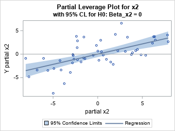
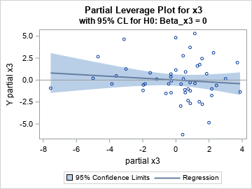
data Have;
set sashelp.iris(
    rename=(PetalLength = Y
            PetalWidth  = x1
            SepalLength = x2
            SepalWidth  = x3)
    where=(Species="Versicolor"));
label Y= x1= x2= x3=;
run;
 
proc reg data=Have plots(only)=PartialPlot;
   model Y = x1 x2 x3 / clb partial partialdata;
   ods exclude PartialPlotData;
   ods output PartialPlotData=PD;
quit;
 
/* macro to create a partial leverage plot (with CLM) for each variable */
%macro MakePartialPlot(VarName);
   title "Partial Leverage Plot for &VarName";
   title2 "with 95% CL for H0: Beta_&VarName = 0";
   proc sgplot data=PD ;
      reg     y=part_Y_&VarName x=part_&VarName / CLM;
      refline 0 / axis=y;
   run;
%mend;
 
%MakePartialPlot(x2);
%MakePartialPlot(x3);

Confidence limits on a partial leverage plot: The efficient way

The previous section shows an easy way to produce partial leverage regression plots in SAS. The confidence bands are a graphical way to examine the null hypotheses β_i = 0. Look at the confidence band for the partial leverage plot for the X2 variable. The Y=0 axis (the gray line) is NOT wholly contained in the confidence band. You can therefore reject (with 95% confidence) the null hypotheses that β₂=0. In contrast, look at the confidence band for the partial leverage plot for the X3 variable. The Y=0 axis IS wholly contained in the confidence band. You therefore cannot reject the null hypotheses that β₃=0.

Although this method is easy, Sall (1990) points out that it is not the most computationally efficient method. For every variable, the SGPLOT procedure computes a bivariate regression, which means that this method requires performing k+2 linear regressions: the regression for the original data that has k regressors, followed by additional bivariate regression for the intercept and each of the k regressors. In practice, each bivariate regression can be computed very quickly, so the entire process is not very demanding. Nevertheless, Sall (1990) showed that all the information you need is already available from the regression on the original data. You just need to save that information and use it to construct the confidence bands.

The following section uses Sall's method to compute the quantities for the partial leverage plots. The program is included for the mathematically curious; I do not recommend that you use it in practice because the previous method is much simpler.

Sall's method for computing partial leverage regression plots

Sall's method requires the following output from the original regression model:

• The means of the regressor variables. You can get these statistics by using the SIMPLE option on the PROC REG statement and by using ODS OUTPUT SimpleStatistics=Simple to save the statistics to a data set.
• The inverse of the crossproduct matrix (the X`*X matrix). You can get this matrix by using the I option on the MODEL statement and by using ODS OUTPUT InvXPX=InvXPX to save the matrix to a data set.
• The mean square error and the error degrees of freedom for the regression model. You can get these statistics by using ODS OUTPUT ANOVA=Anova to save the ANOVA table to a data set.
• The parameter estimates and the F statistics for the null hypotheses β_i=0. You can get these statistics by using the CLB option on the MODEL statement and by using ODS OUTPUT ParameterEstimates=PE to save the parameter estimates table to a data set. The data set contains t statistics for the null hypotheses, but the F statistic is the square of the t statistic.

The following call to PROC REG requests all the statistics and saves them to data sets:

proc reg data=Have plots(only)=PartialPlot simple;
   model Y = x1 x2 x3 / clb partial partialdata I;
   ods exclude InvXPX PartialPlotData;
   ods output SimpleStatistics=Simple
              InvXPX=InvXPX ANOVA=Anova ParameterEstimates=PE 
              PartialPlotData=PD(drop=Model Dependent Observation);
quit;

Sall (1990) shows how to use these statistics to create the partial leverage plots. The following SAS/IML program implements Sall's method.

/* Add confidence bands to partial leverage plots: 
   Sall, J. P. (1990). "Leverage Plots for General Linear Hypotheses."  
   American Statistician 44:308–315.
*/
proc iml;
alpha = 0.05;
 
/* Use statistics from original data to estimate the confidence bands */
/* xBar = mean of each original variable */
use Simple;  read all var "Mean" into xBar; close;
p = nrow(xBar)-1;            /* number of parameters */
xBar = xBar[1:p];            /* remove the Y mean */
 
/* get (X`*X)^{-1} matrix */
use InvXPX;  read all var _NUM_ into xpxi;  close;
xpxi = xpxi[1:p, 1:p];       /* remove column and row for Y */
hbar = xbar` * xpxi * xbar;  /* compute hbar from inv(X`*X) and xbar */
 
/* get s2 = mean square error and error DF */
use ANOVA;  read all var {DF MS};  close;
s2 = MS[2];                  /* extract MSE */
DFerror = DF[2];             /* extract error DF */
 
/* get parameter estimates and t values */
use PE;  read all var {Estimate tValue};  close;
FValue  = tValue#tValue;     /* F statistic is t^2 for OLS */
b = Estimate;                /* lines have slope b[i] and intercept 0 */
 
tAlpha  = quantile("T", 1-alpha/2, DFerror); /* assume DFerror > 0 */
FAlpha  = tAlpha#tAlpha;     /* = quantile( "F", 1-alpha, 1, DFerror); */
 
/* Get partial plot data from REG output */
/* read in part_: names for intercept and X var names */
use PD;  read all var _NUM_ into partial[c=partNames];  close;
 
/* The formula for the confidence limits is from Sall (1990) */
nPts = 100;               /* score CL at nPts values on [xMin, xMax] */ 
XPts = j(nPts, p, .);     /* allocate matrices to store the results  */
Pred  = j(nPts, p, .);
Lower = j(nPts, p, .);
Upper = j(nPts, p, .);
do i = 1 to p;
   levX = partial[,2*i-1];               /* partial x variable */
   xMin = min(levX);  xMax = max(levX);  /* [xMin, xMax] */
   /* partial regression line is (t,z) and CL band is (t, z+/- SE) */
   t = T( do(xMin,xMax,(xMax-xMin)/(nPts-1)));   /* assume xMin < xMax */
   z = b[i]*t;                                   /* predicted mean: yHat = b[i]*x + 0 */
   SE = sqrt( s2#FAlpha#hbar + FAlpha/FValue[i] # (z#z) ); /* Sall, 1990 */
   XPts[,i] = t;
   Pred[,i]  = z;
   Lower[,i] = z - SE;
   Upper[,i] = z + SE;
end;
 
/* create names for new variables for the CL band */
oddIdx = do(1,ncol(partNames),2);  /* names we want are the ODD elements */
Names = partNames[,oddIdx];
XNames     = compress('X_'   +Names);
PredNames  = compress('Pred_'+Names);
LowerNames = compress('LCL_' +Names);
UpperNames = compress('UCL_' +Names);
 
/* write regression lines and confidence bands to a data set */
Results = XPts || Pred || Lower || Upper;
create PartCL from Results[c=(XNames||PredNames||LowerNames||UpperNames)];
   append from Results;
close; 
QUIT;

The data set PartCL contains the fit lines (which have slopes equal to b[i]) and the lower and upper confidence limits for the means of the partial leverage plots. The lines are evaluated at 100 evenly spaced points in the range of the "partial variables." The program uses matrix multiplication to evaluate the quadratic form $\bar{x}^\prime (X^\prime X)^{-1} \bar{x}$. The remaining computations are scalar operations.

The following statements merge the regression lines and confidence intervals with the data for the partial leverage plots. You can then create a scatter plot of the partial leverage values and overlay the regression line and confidence bands.

data Want;
set PD PartCL;
run;
 
/* macro for plotting a partial leverage plot with CL from the IML program */
%macro MakePartialPlotCL(VarName);
   title "Partial Leverage Plot for &VarName";
   proc sgplot data=Want noautolegend;
      band    x=x_part_&VarName lower=LCL_part_&VarName upper=UCL_part_&VarName; 
      scatter x=part_&VarName y=part_Y_&VarName;
      series  x=x_part_&VarName y=Pred_part_&VarName;
      refline 0 / axis=y;
   run;
%mend;
 
ods graphics / PUSH AttrPriority=None width=360px height=270px;
%MakePartialPlotCL(x2);
%MakePartialPlotCL(x3);
ods graphics / POP;      /* restore ODS GRAPHICS options */

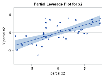
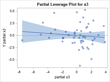
As expected, the graphs are the same as the ones in the previous section. However, the quantities in the graphs are all produced by PROC REG as part of the computations for the original regression model. No additional regression computations are required.

Summary

This article shows two ways to get a confidence band for the conditional mean of a partial regression plot. The easy way is to use the REG statement in PROC SGPLOT. A more efficient way is to compute the confidence band directly from the statistics on the original data. This article shows how to use the SAS/IML language to compute the confidence limits from the output of PROC REG.

This article also demonstrates a key reason why SAS customers choose SAS/IML software. They want to compute some statistic that is not directly produced by any SAS procedure. The SAS/IML language enables you to combine the results of SAS procedures and use matrix operations to compute other statistics from formulas in textbooks or journal articles. In this case, PROC IML consumes the output of PROC REG and creates regression lines and confidence bands for partial leverage plots.