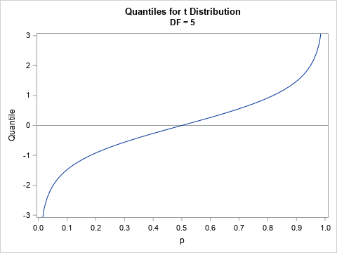
Recently, I needed to solve an optimization problem in which the objective function included a term that involved the quantile function (inverse CDF) of the t distribution, which is shown to the right for DF=5 degrees of freedom. I casually remarked to my colleague that the optimizer would have to use finite-difference derivatives because "this objective function does not have an analytical derivative." But even as I said it, I had a nagging thought in my mind. Is that statement true?

I quickly realized that I was wrong. The quantile function of ANY continuous probability distribution has an analytical derivative as long as the density function (PDF) is nonzero at the point of evaluation. Furthermore, the quantile function has an analytical expression for the second derivative if the density function is differential.

This article derives an exact analytical expression for the first and second derivatives of the quantile function of any probability distribution that has a smooth density function. The article demonstrates how to apply the formula to the t distribution and to the standard normal distribution. For the remainder of this article, we assume that the density function is differentiable.

The derivative of a quantile function

It turns out that I had already solved this problem in a previous article in which I looked at a differential equation that all quantile functions satisfy. In the appendix of that article, I derived a relationship between the first derivative of the quantile function and the PDF function for the same distribution. I also showed that the second derivative of the quantile function can be expressed in terms of the PDF and the derivative of the PDF.

Here are the results from the previous article. Let X be a random variable that has a smooth density function, f. Let w = w(p) be the p_th quantile. Then the first derivative of the quantile function is
$\frac{dw}{dp} = \frac{1}{f(w(p))}$
provided that the denominator is not zero. The second derivative is
$\frac{d^2w}{dp^2} = \frac{-f^\prime(w)}{f(w)} \left( \frac{dw}{dp} \right)^2 = \frac{-f^\prime(w)}{f(w)^3}$.

Derivatives of the quantile function for the t distribution

Let's confirm the formulas for the quantile function of the t distribution with five degrees of freedom. You can use the PDF function in SAS to evaluate the density function for many common probability distributions, so it is easy to get the first derivative of the quantile function in either the DATA step or in the IML procedure, as follows:

proc iml;
reset fuzz=1e-8;
DF = 5;
/* first derivative of the quantile function w = F^{-1}(p) for p \in (0,1) */
start DTQntl(p) global(DF);
   w = quantile("t", p, DF);  /* w = quantile for p */
   fw = pdf("t", w, DF);      /* density at w */
   return( 1/fw );
finish;
 
/* print the quantile and derivative at several points */
p = {0.1, 0.5, 0.75};
Quantile = quantile("t", p, DF);  /* w = quantile for p */
DQuantile= DTQntl(p);
print p Quantile[F=Best6.] DQuantile[F=Best6.];

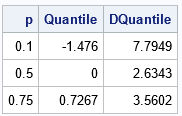
This table shows the derivative (third column) for the quantiles of the t distribution. If you look at the graph of the quantile function, these values are the slope of the tangent lines to the curve at the given values of the p variable.

Second derivatives of the quantile function for the t distribution

With a little more work, you can obtain an analytical expression for the second derivative. It is "more work" because you must use the derivative of the PDF, and that formula is not built-in to most statistical software. However, derivatives are easy (if unwieldy) to compute, so if you can write down the analytical expression for the PDF, you can write down the expression for the derivative.

For example, the following expression is the formula for the PDF of the t distribution with ν degrees of freedom:

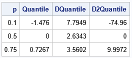
/* derivative of the PDF for the t distribution */
start Dtpdf(x) global(DF);
   nu = DF;
   pi = constant('pi');
   A = Gamma( (nu +1)/2 ) / (sqrt(nu*pi) * Gamma(nu/2));
   dfdx = A * (-1-nu)/nu # x # (1 + x##2/nu)##(-(nu +1)/2 - 1); 
   return dfdx;
finish;
 
/* second derivativbe of the quantile function for the t distribution */
start D2TQntl(p) global(df);
   w = quantile("t", p, df);
   fw = pdf("t", w, df);
   dfdx = Dtpdf(w);
   return( -dfdx / fw##3 );
finish;
 
D2Quantile = D2TQntl(p);
print p Quantile[F=Best6.] DQuantile[F=Best6.] D2Quantile[F=Best6.];

Derivatives of the normal quantiles

You can use the same theoretical formulas for the normal quantiles. The second derivative, however, does not require that you compute the derivative of the normal PDF. It turns out that the derivative of the normal PDF can be written as the product of the PDF and the quantile function, which simplifies the computation. Specifically, if f is the standard normal PDF, then $f^\prime(w) = -f(w) w$.
and so the second derivative of the quantile function is
$\frac{d^2w}{dp^2} = w \left( \frac{dw}{dp}\right)^2$.
This is shown in the following program:

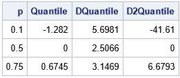
/* derivatives of the quantile function for the normal distribution */ proc iml; /* first derivative of the quantile function */ start DNormalQntl(p); w = quantile("Normal", p); fw = pdf("Normal", w); return 1/fw; finish; /* second derivative of the quantile function */ start D2NormalQntl(p); w = quantile("Normal", p); dwdp = DNormalQntl(p); return( w # dwdp##2 ); finish;   p = {0.1, 0.5, 0.75}; Quantile = quantile("Normal", p); DQuantile = DNormalQntl(p); D2Quantile = D2NormalQntl(p); print p Quantile[F=Best6.] DQuantile[F=Best6.] D2Quantile[F=Best6.];

Summary

In summary, this article shows how to compute the first and second derivatives of the quantile function for any probability distribution (with mild assumptions for the density function). The first derivative of the quantile function can be defined in terms of the quantile function and the density function. For the second derivative, you usually need to compute the derivative of the density function. The process is demonstrated by using the t distribution. For the standard normal distribution, you do not need to compute the derivative of the density function; the derivatives depend only on the quantile function and the density function.