M estimation is a robust regression technique that assigns a weight to each observation based on the magnitude of the residual for that observation. Large residuals are downweighted (assigned weights less than 1) whereas observations with small residuals are given weights close to 1. By iterating the reweighting and fitting steps, the method converges to a regression that de-emphasizes observations whose residuals are much bigger than the others. This iterative process is also known called iteratively reweighted least squares.
A previous article visualizes 10 different "weighting functions" that are supported by the ROBUSTREG procedure in SAS. That article mentions that the results of the M estimation process depend on the choice of the weighting function. This article runs three robust regression models on the same data. The only difference between the three models is the choice of a weighting function. By comparing the regression estimates for each model, you can understand how the choice of a weighting function affects the final model.
Data for robust regression
The book Applied Regression Analysis and Generalized Linear Models (3rd Ed, J. Fox, 2016) analyzes Duncan's occupational prestige data (O. D. Duncan, 1961), which relates prestige to the education and income of men in 45 occupations in the US in 1950. The following three variables are in the data set:
- Income (Explanatory): Percent of males in the occupation who earn $3,500 or more.
- Education (Explanatory): Percent of males in the occupation who are high-school graduates.
- Prestige (Response): Percent of raters who rated the prestige of the occupation as excellent or good.
The following scatter plot shows the distributions of the Income and Education variables. The color of the marker reflects the Prestige variable. Certain occupations are labeled:
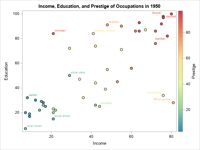
The markers are roughly divided into four regions:
- The cluster of markers in the lower-left corner of the graph are unskilled laborers such as coal miners, truck drivers, and waiters. The men in these occupations have little education and earn little income.
- Markers in the lower-right corner represent are skilled laborers such as plumbers and railroad conductors who make considerable income despite having little education.
- Markers in the upper-left corner represent occupations such as ministers and welfare workers who have considerable education but low-paying jobs.
- Markers in the upper-right corner represent occupations such as doctors, lawyers, and bankers who have a lot of education and high income.
In general, the prestige of an occupation increases from lower-left to upper-right. However, there are some exceptions. A minister has more prestige than might be expected from his income. Reporters and railroad conductors have less prestige than you might expect from their income. A robust regression model that uses M estimation will assign smaller weights to observations that do not match the major trends in the data. Observations that have very small weights are classified as outliers.
The following SAS DATA step creates Duncan's prestige data:
/* Duncan's Occupational Prestige Data from John Fox (2016), Applied Regression Analysis and Generalized Linear Models, Third Edition https://socialsciences.mcmaster.ca/jfox/Books/Applied-Regression-3E/datasets/Duncan.txt Original source: Duncan, O. D. (1961) A socioeconomic index for all occupations. In Reiss, A. J., Jr. (Ed.) Occupations and Social Status. Free Press [Table VI-1]. Type: prof=Professional, wc=White collar, bc=Blue collar */ data Duncan; length Occupation $20 Type $4; input Occupation Type Income Education Prestige; ObsNum + 1; datalines; accountant prof 62 86 82 pilot prof 72 76 83 architect prof 75 92 90 author prof 55 90 76 chemist prof 64 86 90 minister prof 21 84 87 professor prof 64 93 93 dentist prof 80 100 90 reporter wc 67 87 52 engineer prof 72 86 88 undertaker prof 42 74 57 lawyer prof 76 98 89 physician prof 76 97 97 welfare.worker prof 41 84 59 teacher prof 48 91 73 conductor wc 76 34 38 contractor prof 53 45 76 factory.owner prof 60 56 81 store.manager prof 42 44 45 banker prof 78 82 92 bookkeeper wc 29 72 39 mail.carrier wc 48 55 34 insurance.agent wc 55 71 41 store.clerk wc 29 50 16 carpenter bc 21 23 33 electrician bc 47 39 53 RR.engineer bc 81 28 67 machinist bc 36 32 57 auto.repairman bc 22 22 26 plumber bc 44 25 29 gas.stn.attendant bc 15 29 10 coal.miner bc 7 7 15 streetcar.motorman bc 42 26 19 taxi.driver bc 9 19 10 truck.driver bc 21 15 13 machine.operator bc 21 20 24 barber bc 16 26 20 bartender bc 16 28 7 shoe.shiner bc 9 17 3 cook bc 14 22 16 soda.clerk bc 12 30 6 watchman bc 17 25 11 janitor bc 7 20 8 policeman bc 34 47 41 waiter bc 8 32 10 ; |
Analysis 1: The bisquare weighting function
The following call to PROC ROBUSTREG shows how to run a robust regression analysis of the Duncan prestige data. The METHOD=M option tells the procedure to use M estimation. The WEIGHTFUNCTION= suboption specifies the weight function that will assign weights to observations based on the size of the residuals.
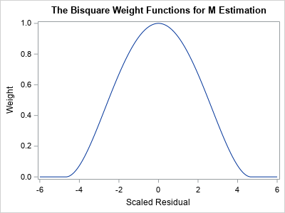
The default weight function is the bisquare function, but the following statements specify the weight function explicitly. A graph of the bisquare weighting function is shown to the right. Observations that have a small residual receive a weight near 1; outliers receive a weight close to 0.
title "Robust Regression Analysis for WEIGHTFUNCTION=Bisquare"; proc robustreg data=Duncan plots=RDPlot method=M(WEIGHTFUNCTION=Bisquare); model Prestige = Income Education; ID Occupation; output out=RROut SResidual=StdResid Weight=Weight Leverage=Lev Outlier=Outlier; ods select ParameterEstimates RDPlot; run; |
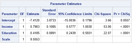
The parameter estimates are shown. The bisquare-weighted regression model is
Prestige = -7.41 + 0.79*Income + 0.42*Education.
The intercept term is not significant at the 0.05 significance level, so you could rerun the analysis to use a no-intercept model. We will not do that here.
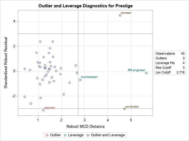
The plot is called the residual-distance plot (RD plot). You can use an RD plot to identify high-leverage points and outliers for the model. This is a robust version of the residual-leverage plot that is used for ordinary least-squares regression.
- The horizontal direction is a robust measure of the leverage. Think of it as a robust distance from the coordinates of each observation to a robust estimate of the center of the explanatory variables. Observations that have a large distance are high-leverage points. M estimation is not robust to the presence of high-leverage points, so SAS will display a WARNING in the log that states "The data set contains one or more high-leverage points, for which M estimation is not robust." You can see from this plot (or from the scatter plot in the previous section) that bookkeepers, ministers, conductors, and railroad engineers are somewhat far from the center of the point cloud in the bivariate space of the explanatory variables (Income and Education). Therefore, they are high-leverage points.
- The vertical direction shows the size of a standardized residual for the robust regression model. Reference lines are drawn at ±3. If an observation has a residual that exceeds these values, it is considered an outlier, meaning that the value of Prestige in the data is much higher or lower than the value predicted by the model. You can see from this plot that ministers, reporters, and conductors are outliers for this model.
The graph of the bisquare weighting function enables you to mentally estimate the weights for each observation. But an easier way to visualize the weights is to use the WEIGHT= option on the OUTPUT statement to output the weights to a SAS data set. You can then plot the weight for each observation and label the markers that have small weights, as follows:
data RROut2; set RROut; length Label $20; if Weight < 0.8 then Label = Occupation; else Label = ""; run; title "Weights for WEIGHTFUNCTION=Bisquare"; proc sgplot data=RROut2; scatter x=ObsNum y=Weight / datalabel=Label; run; |
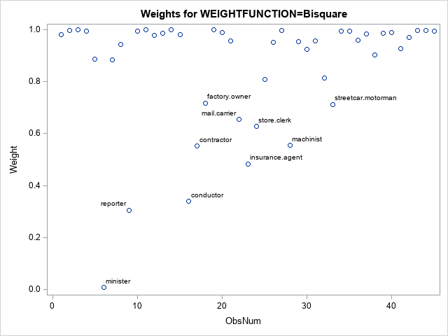
The scatter plot (click to enlarge) shows the weights for all observations. A few that have small weights (including the outliers) are labeled. You can see that the minister has a weight close to Weight=0 whereas reporters and conductors have weights close to Weight=0.3. These weights are used in a weighted regression, which is the final regression model.
If you prefer a tabular output, you can use the LEVERAGE= and OUTLIER= options on the OUTPUT statement to output indicator variables that identify each observation as a high-leverage point, an outlier, or both. The following call to PROC PRINT shows how to display only the outliers and high-leverage points:
proc print data=RROut; where Lev=1 | Outlier=1; var Occupation Weight Prestige Income Education Lev Outlier; run; |
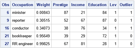
The output shows that four observations are high-leverage points and three are outliers. (The minister and reporter occupations are classified as both.) This outlier classification depends on the weighting function that you use during the M estimation procedure.
Create a SAS macro to repeat the analysis
You can repeat the previous analysis for other weighting functions to see how the choice of a weighting function affects the final regression fit. It makes sense to wrap up the main functionality into a SAS macro that takes the name of the weighting function as an argument, as follows:
%macro RReg( WeightFunc ); title "Robust Regression Analysis for WEIGHTFUNCTION=&WeightFunc"; proc robustreg data=Duncan plots=RDPlot method=M(WEIGHTFUNCTION=&WeightFunc); model Prestige = Income Education; ID Occupation; output out=RROut SResidual=StdResid Weight=Weight; ods select ParameterEstimates RDPlot; run; data RROut2; set RROut; length Label $20; if Weight < 0.8 then Label = Occupation; else Label = ""; run; title "Weights for WEIGHTFUNCTION=&WeightFunc"; proc sgplot data=RROut2; scatter x=ObsNum y=Weight / datalabel=Label; run; %mend; |
The next sections call the macro for the Huber and Talworth weighting functions, but you can use it for any of the 10 weighting functions that PROC ROBUSTREG supports.
Analysis 2: The Huber weighting function
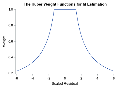
A graph of the Huber weight function is shown to the right. Notice that the any observation whose standardized residual is less than 1.345 receives a weight of 1. Observations that have larger residuals are downweighted by using a weight that is inversely proportional to the magnitude of the residual.
The following statement re-runs the M estimation analysis, but uses the Huber weighting function:
%RReg( Huber ); |
The parameter estimates are not shown, but the Huber-weighted regression model is
Prestige = -7.1107 + 0.70*Income + 0.49*Education.
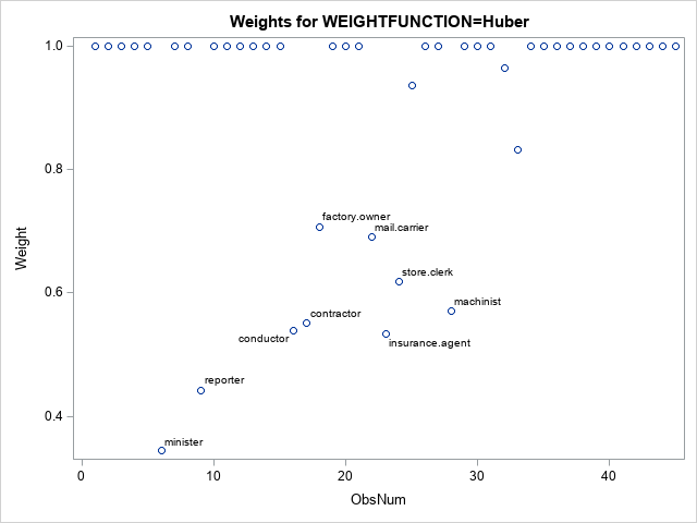
Notice that the estimates are different from the bisquare analysis because the Huber and bisquare functions result in different weights.
For this model, reporters and ministers are outliers. Many observations receive full weight (Weight=1) in the analysis. A handful of observations are downweighted, as shown in the following scatter plot (click to enlarge):
Analysis 3: The Talworth weighting function
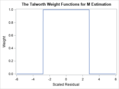
A graph of the Talworth weight function is shown to the right. Notice that any observation whose standardized residual is less than 2.795 receives a weight of 1. All other observations are excluded from the analysis by assigning them a weight of 0.
The following statement re-runs the M estimation analysis, but uses the Talworth weighting function:
%RReg( Talworth ); |
The parameter estimates are not shown, but the Talworth-weighted regression model is
Prestige = -7.45 + 0.74*Income + 0.46*Education.
Again, the estimates are different from the estimates that used the other weighting functions.
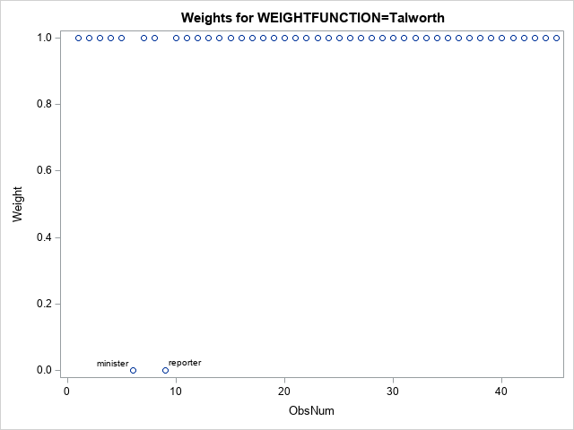
For this analysis, the reporters and ministers are outliers. All other observations receive Weight=1. The weights are shown in the following scatter plot (click to enlarge):
Summary
Many statistical procedures depend on parameters, which affect the results of the procedure. Users of SAS software often accept the default methods, but it is important to recognize that an analysis can and will change if you use different parameters. For the ROBUSTREG procedure, the default method is M estimation, and the default weighting function is the bisquare weighting function. This article demonstrates that the fitted regression model will change if you use a different weighting function. Different weighting functions can affect which observations are classified as outliers. Each function assigns different weights to observations that have large residual values.
