Many modern statistical techniques incorporate randomness: simulation, bootstrapping, random forests, and so forth. To use the technique, you need to specify a seed value, which determines pseudorandom numbers that are used in the algorithm. Consequently, the seed value also determines the results of the algorithm. In theory, if you know the seed value and the internal details of the pseudorandom algorithm, then the stream is completely determined, and the results of an algorithm are reproducible. For example, if I publish code for a simulation or bootstrap method in SAS, you can reproduce my computations as long as my program specifies the seed value for every part of the program that uses random numbers.

Occasionally, programmers post questions on discussion forums about how to compare the results that were obtained by using different software. A typical question might be, "My colleague used R to run a simulation. He gets a confidence interval of [14.585, 21.42]. When I run the simulation in SAS, I get [14.52, 21.19]. How can I get the same results as my colleague?" In most cases, you can't get the same answer. More importantly, it doesn't matter: these two results are equally valid estimates. When you run an algorithm that uses pseudorandom numbers, you don't get THE answer, you get AN answer. There are many possible answers you can get. Each time you change the random number stream, you will get a different answer, but all answers are equally valid.

This article examines how the random number seed affects the results of a bootstrap analysis by using an example of a small data set that has N=10 observations. I will run the same bootstrap analysis for 50 different seeds and compare the results of a confidence interval. The same ideas apply to simulation studies, machine learning algorithms, and other algorithms that use randomness to obtain an answer.

A bootstrap estimate of a confidence interval

The following data were used by Davison, Hinkley, and Schechtman (1986). They ran an analysis to examine the bootstrap distribution of the sample mean in a small nonnormal set of data. The goal of the following analysis is to obtain a bootstrap estimate of a 90% confidence interval for the population mean. Because we are going to run the same analysis many times with different random number seeds, I will put the bootstrap steps in a SAS macro. The following statements run two bootstrap analyses on the same data. The only difference is the value of the random-number seeds.

data Sample;
input x @@;
datalines;
9.6 10.4 13.0 15.0 16.6 17.2 17.3 21.8 24.0 33.8
;
 
/* macro to perform one bootstrap analysis that uses NumSamples resamples
   and uses a particular seed. Results are in the data set BootEst */
%macro Do1Boot(seed, NumSamples);
   /* 1. generate NumSamples bootstrap resamples from SEED value */
   proc surveyselect data=Sample NOPRINT seed=&SEED
        method=urs              /* URS = resample with replacement */
        samprate=1              /* each bootstrap sample has N obs */
        OUTHITS                 /* do not use a frequency var */
        reps=&NumSamples(repname=SampleID)        /* generate NumSamples samples */
        out=BootSamp;
   run;
 
   /* 2. compute sample mean for each resample; write to data set */
   proc means data=BootSamp NOPRINT;
      by SampleID;
      var x;
      output out=BootStats mean=Mean;  /* bootstrap distribution */
   run;
   /* 3. find boostrap estimates of mean, stdErr, and 90% CI */
   proc means data=BootStats NOPRINT;
      var Mean;
      output n=N mean=Mean stddev=StdErr p5=LCL90 p95=UCL90
             out=BootEst(drop=_TYPE_ _FREQ_);
   run;
   /* add the seed value to these statistics */
   data BootEst;
      Seed = &seed;
      set BootEst;
   run;
%mend;
 
title "A Boostrap Analysis for Seed=1";
%Do1Boot(1, 1000);
proc print data=BootEst noobs; run;
 
title "A Boostrap Analysis for Seed=1234";
%Do1Boot(1234, 1000);
proc print data=BootEst noobs; run;

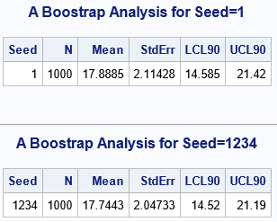
The output shows that the bootstrap estimates are similar, but not exactly the same. This is expected. Each analysis uses a different seed, which means that the bootstrap resamples are different between the two runs. Accordingly, the means of the resamples are different, and so the bootstrap distributions are different. Consequently, the descriptive statistics that summarize the bootstrap distributions will be different. To make the differences easier to see, I used only 1,000 samples in each bootstrap analysis. If you increase the number of resamples to, say, 10,000, the differences between the two analyses will be smaller.

The fact that the random number seed "changes" the result makes some people nervous. Which value should you report to a journal, to a customer, or to your boss? Which is "the right answer"?

Both answers are correct. A bootstrap analysis relies on randomness. The results from the analysis depend on the pseudorandom numbers that are used.

Do the results depend on the seed value?

You should think of each bootstrap estimate as being accurate to some number of digits, where the number of digits depends on the number of resamples, B. For some estimates, such as the bootstrap standard error, you can calculate that the accuracy is proportional to 1/sqrt(B). Thus, larger values for B tend to shrink the difference between two bootstrap analyses that use different random number streams.

One way to visualize the randomness in a bootstrap estimate is to run many bootstrap analyses that are identical except for the random-number seed. The following SAS macro runs 50 bootstrap analyses and uses the seed values 1,2,3,..., 50:

/* Run nTrials bootstrap analyses. The i_th trials uses SEED=i. The estimates are written 
   to the data set AllBoot by concatenating the results from each analysis. */
%macro DoNBoot(NumSamples, nTrials);
   options nonotes;
   proc datasets noprint nowarn;   /* delete data set */
      delete AllBoot;
   quit;
   %do seed = 1 %to &nTrials;
       %Do1Boot(&seed, &numSamples);   /* run with seed=1,2,3,...,nTrials */
       proc append base=AllBoot data=BootEst force; 
       run;
   %end;
   options notes;
%mend;
 
/* Run 50 bootstrap analyses: numSamples=1000, nTrials=50, seeds=1,2,3,...,50 */
%DoNBoot(1000, 50); 
 
/* find boostrap estimates of mean, stdErr, and 90% CI */
title "Variation in 50 Traditional Boostrap Estimates";
proc means data=AllBoot N Mean StdDev Min Max;
   var Mean StdErr LCL90 UCL90;
run;

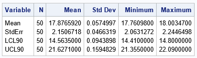
The table shows how four estimates vary across the 50 bootstrap analyses:

• The bootstrap estimate of the mean varies in the interval [17.76, 18.00]. The average of the 50 estimates is 17.88.
• The bootstrap estimate of the standard error varies in the interval [2.06, 2.25]. The average of the 50 estimates is 17.88.
• The bootstrap estimate of the lower 90% confidence interval varies in the interval [14.41, 14.80]. The average of the 50 estimates is 14.56.
• The bootstrap estimate of the upper 90% confidence interval varies in the interval [21.36, 22.09]. The average of the 50 estimates is 21.63.

The table shows that the variation among the 50 estimates is small (and can be made smaller by increasing B). If you and your colleague run an identical bootstrap analysis but use different seed values, you are likely to obtain results that are similar to each other. Even more comforting is that the inferences that you make from the analyses should be the same. For example, suppose you are testing the null hypotheses that these data came from a population in which the mean is μ=20. Let's look at the 90% confidence intervals for the 50 analyses:

title "Traditional Bootstrap Estimates";
title2 "Varying Seed Values";
proc sgplot data=AllBoot;
   refline &ObsStat / axis=Y label="Sample Mean";
   highlow x=Seed low=LCL90 high=UCL90 / legendlabel="90% CL";
   scatter x=Seed y=Mean / legendlabel="Bootstrap Estimate";
   yaxis label="x" ;
run;

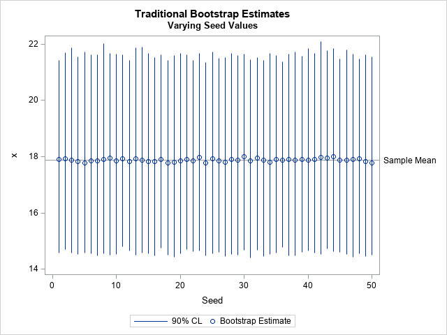
The graph shows that the value μ=20 is inside all 50 of the confidence intervals. Therefore, the decision to accept or reject the null hypothesis does not depend on the seed value when μ=20.

On the other hand, if you are testing whether the population mean is μ=21.5, then some analyses would reject the null hypothesis whereas others would fail to reject it. What to do in that situation? I would acknowledge that there is uncertainty in the inference and conclude that it cannot be reliably decided based on these data and these analyses. It would be easy to generate additional bootstrap samples (increase B). You could also advocate for collecting additional data, if possible.

Summary

In summary, the result of a bootstrap analysis (and ANY statistical technique that uses randomness) depends on the stream of pseudorandom numbers that are used. If you change the seed or use different statistical software, you are likely to obtain a different result, but the two results should be similar in many cases. You can repeat the analysis several times with different seeds to understand how the results vary according to the random-number seed.

If some seed values enable you to reject a hypothesis and others do not, you should acknowledge that fact. It is not ethical to use the seed value that gives the result that you want to see! (See "How to lie with a simulation" for an example.)

If you are nervous about the result of an algorithm that uses randomness, I suggest that you rerun the analysis several times with different seed values. If the results are consistent across seeds, then you can have confidence in the analysis. If you get vastly different results, then you are justified in being nervous.