How to unroll frequency data

In categorical data analysis, it is common to analyze tables of counts. For example, a researcher might gather data for 18 boys and 12 girls who apply for a summer enrichment program. The researcher might be interested in whether the proportion of boys that are admitted is different from the proportion of girls. For this analysis, the data that you type into statistical software (such as SAS) does not typically consist of 20 observations. Rather, the data often consists of four observations and a frequency variable (also call a count variable). The first two observations record the number of boys that are admitted and not admitted, respectively. The next two observations record the corresponding frequencies for the girls. This representation of the data is sometimes called frequency data. It is used when you can group individual subjects into categories such as boy/girl and admitted/not admitted. Despite its convenience, there are times when it is useful to expand or "unroll" the data to enumerate the individual subjects. Examples include bootstrap estimates and analyzing the data in SAS procedures that do not support a FREQ statement. This article shows how to use the SAS DATA step to unroll frequency data. In addition, this article shows how to expand data that are in events/trials format.

Data in frequency form

The following example is from the documentation of the FREQ procedure. The goal is to compute some statistics for a 2 x 2 frequency table for 23 patients. Eight patients were on a low-cholesterol diet and 15 were on a high-cholesterol diet. The table shows how many subjects in each group developed heart disease. The data are used to estimate the relative risk of developing heart disease in the two groups:

/* Doc Example: PROC FREQ analysis of a 2x2 Contingency Table */
proc format;
   value ExpFmt 1='High Cholesterol Diet'  0='Low Cholesterol Diet';
   value RspFmt 1='Yes'  0='No';
run;
 
data FatComp;
format Exposure ExpFmt. Response RspFmt.;
input Exposure Response Count;
label Response='Heart Disease';
datalines;
0 0  6
0 1  2
1 0  4
1 1 11
;
 
title 'Case-Control Study of High Fat/Cholesterol Diet';
proc freq data=FatComp;
   tables Exposure*Response / relrisk norow nocol nopercent;
   weight Count;            /* each row represents COUNT patients */
run;

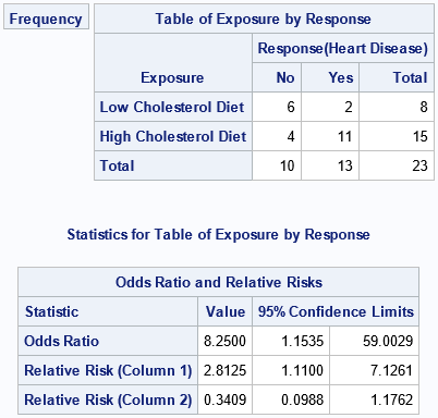
Notice that the data are input in terms of group frequencies. The output is shown. The analysis estimates the risk of heart disease for a subject on a high-cholesterol diet as 2.8 times greater than the risk for a subject on a low-cholesterol diet.

How to unroll frequency data in SAS

You can use the DATA step in SAS to unroll the frequency data. The COUNT variable tells you how many patients are in each group. You can therefore write a loop that expands the data: iterate from 1 to the COUNT value and put an OUTPUT statement in the body of the loop. If desired, you can include an ID variable to enumerate the subjects in each group, as follows:

data RawFat;
set FatComp;
Group + 1;          /* identify each category */
do ID = 1 to Count; /* identify subjects in each category */
   output;
end;
drop Count;
run;
 
proc print data=RawFat(obs=10);
run;

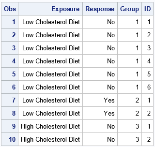
Whereas the original data set has four rows, the RawFat data has 23 rows. The first 10 rows are shown. The first six observations are the expansion of the subjects in the first group (Exposure=Low; Response=No). The next two observations are the subjects in the second group (Exposure=Low; Response=Yes), and so forth. The GROUP variable identifies the original groups. The ID variable enumerates patients within each group. The second data set can be analyzed by any SAS procedure. In this form, the data do not require using a FREQ statement (or the WEIGHT statement in PROC FREQ), as shown by the following call to PROC FREQ:

/* run the same analysis on the expanded data */
proc freq data=RawFat;
   tables Exposure*Response / relrisk norow nocol nopercent;
   /* no WEIGHT statement because there is one row for each patient */
run;

The output (not shown) is the same as for the frequency data. Both data sets contain the same information, but the second might be useful for certain tasks such as a bootstrap analysis.

Data in events/trials form

A related data format is called the events/trials format. In the events/trials format, each observation has two columns that specify counts. One column specifies the number of times that a certain event occurs, and the other column specifies the number of trials (or attempts) that were conducted. This format is used for logistic regression and for other generalized linear regression models that predict the proportion of events. The following example is from the documentation for the LOGISTIC procedure. The data describe the result of 19 batches of ingots in a designed experiment. Each batch was soaked and heated for specified combinations of times. The ingots were then inspected to determine which were not ready for rolling. The following DATA step records the results in the events/trials syntax. The R variable records the number of ingots that are not ready for rolling, and the N variable contains the number of ingots in the batch at the given values of the HEAT and SOAK variables. Consequently, R/N is the proportion of ingots that were not ready. For example, the values R=4 and N=44 means that 4 ingots (9%) were not ready for rolling in a batch that contained 44. Regression procedures such as PROC LOGISTIC enable you to analyze data by using an events/trials syntax:

/* events/trials syntax */
data ingots;
   input Heat Soak r n @@;
   datalines;
7 1.0 0 10  14 1.0 0 31  27 1.0 1 56  51 1.0 3 13
7 1.7 0 17  14 1.7 0 43  27 1.7 4 44  51 1.7 0  1
7 2.2 0  7  14 2.2 2 33  27 2.2 0 21  51 2.2 0  1
7 2.8 0 12  14 2.8 0 31  27 2.8 1 22  51 4.0 0  1
7 4.0 0  9  14 4.0 0 19  27 4.0 1 16
;
 
proc logistic data=ingots;
   model r/n = Heat Soak;
   ods select NObs ResponseProfile ParameterEstimates;
run;

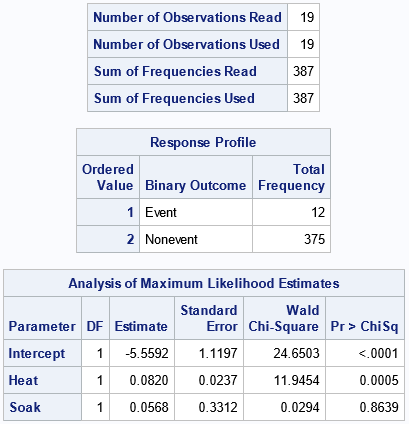
The "NObs" table shows that there are 19 rows of data, which represents 387 units. The "Response Profile" table counts and displays the number of events and the number of trials. For these data, 12 units were not ready for rolling. The "ParameterEstimates" table provides estimates for the Intercept and the coefficients of the effects in the logistic regression model.

How to expand event/trials data

You can expand these data by creating 387 observations, one for each unit. The following DATA step creates a variable named BATCH that enumerates the original 19 batches of ingots. The ID variable enumerates the units in each batch. Some of the units were ready for rolling and some were not. You can create an indicator variable (NOTREADY) that arbitrarily sets the first R ingots as "not ready" (NOTREADY=1) and the remaining ingots as ready (NOTREADY=0).

/* expand or unroll the events/trials data */
data RawIngots;
set ingots;
BatchID + 1;
do ID = 1 to n;
   NotReady = (ID <= r);
   output;
end;
run;
 
/* analyze the binary variable NOTREADY */
proc logistic data=RawIngots;
   model NotReady(event='1') = Heat Soak;
   ods select NObs ResponseProfile ParameterEstimates;
run;

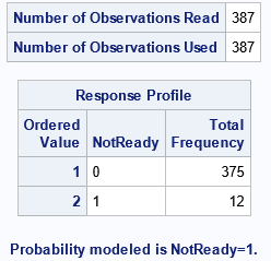
The "NOBs" and "Response Profile" tables are different from before, but they contain the same information. The "ParameterEstimates" table is the same and is not shown.

Summary

In categorical data analysis, it is common to analyze data that are in frequency form. Each observation represents some number of subjects, and the number is given by the value of a Count variable. In some situations, it is useful to "unroll" or expand the data. If an observation has frequency C, it results in C observations in the expanded data set. This article shows how to use the SAS DATA step to expand frequency data and data that are in events/trials syntax.

Blogs