The ERF and ERFC functions for statisticians

Recently, a SAS programmer commented about one of my blog posts. He said that he had found an alternative answer on another website. Whereas my answer was formulated in terms of the normal cumulative distribution function (CDF), the other answer used the ERF function. This article shows the relationship between the normal CDF function, which is favored by statisticians, and the ERF function, which is used by physicists and engineers. Essentially, the two functions are equivalent for computational purposes. This article also shows the relationship between the complementary functions: the normal survival function (SDF) and the complementary ERF function (ERFC).

A familiar function with a strange name

There are many instances where similar topics are given completely different names in different fields of study. An applied mathematician must be multilingual. Here multilingual does not mean being able to speak English, French, Russian, and Chinese, but being able to speak the language of statistics, physics, biology, chemistry. It is also valuable to be able to read and write in multiple computer languages such as SAS, R, Python, C/C++, but that is a different topic!

The ERF function is a sigmoid (S-shaped) function that is defined in terms of an integral. The definition is
ERF(x) = $\frac{2}{\sqrt{\pi}} \int_0^x \exp(-t^2) \, dt$
The constant 2/sqrt(π) normalizes the function so that it approaches 1 as x → ∞. The statistical programmer will note a striking similarity to the standard normal CDF, which is defined as
CDF(x) = $\frac{1}{\sqrt{2\pi}} \int_{-\infty}^x \exp(-t^2/2) \, dt$
Notice that the CDF definition has a lower limit of -∞ and the integrand is exp(-t²/2) rather than exp(-t²).

Compare the ERF function and the normal CDF

The following SAS statements evaluate the ERF and normal CDF functions on the interval [-3, 3] and plot each function:

/* ERF and ERFC functions in SAS */
data ERF;
do x = -3 to 3 by 0.05;
   ERF = erf(x);
   NormCDF = cdf("normal", x);
   output;
end;
run;
 
title "Comparison of ERF and Normal CDF";
proc sgplot data=ERF;
   xaxis grid; yaxis grid display=(nolabel);
   refline 0 / axis=y;
   refline 0 / axis=x;
   series x=x y=ERF / curvelabel curvelabelpos=start;
   series x=x y=NormCDF / curvelabel="CDF" curvelabelpos=start;
run;

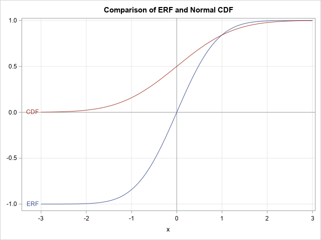
The graph shows that the range of the ERF function is [-1, 1] whereas the range of the CDF function is [0, 1]. In addition, there is a scaling difference: the ERF function is very close to its extreme values for |x| > 2.1, whereas the normal CDF is close to its extreme values for |x| > 3.

From a computational perspective, the two functions are equivalent in the sense that you can transform one function into the other by using only affine transformations. By using a little calculus and algebra, you can show the relationship between the ERF and the normal CDF functions is
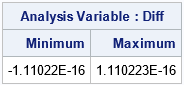
CDF(x) = 1/2 (1 + ERF(x/sqrt(2))). This is shown in the following SAS DATA step, which shows that these two expressions are equal to within machine precision:

data Verify;
do x = -3 to 3 by 0.05;
   ScaledERF = 1/2*(1 + erf(x/sqrt(2)));
   NormCDF = cdf("normal", x);
   Diff = ScaledERF - NormCDF;
   output;
end;
run;
 
proc means data=Verify Min Max;
   var DIff;
run;

Consequently, any formula that can be expressed by using the normal CDF function can also be expressed by using the ERF function, and vice versa. The two functions are computationally equivalent, although the CDF function usually results in cleaner-looking expressions for statistical applications.

The complementary ERF function and the normal survival function

Because the ERF function can be linearly transformed into the normal CDF function, it is no surprise that their complementary functions are also related. The complementary ERF function is defined as ERFC(x) = 1 – ERF(x), and the complementary CDF function (also called the survival function) is defined as SDF(x) = 1 – CDF(x). The following statements graph these functions:

data ERFC;
do x = -3 to 3 by 0.05;
   ERFC = erfc(x);
   NormSDF = sdf("normal", x);
   output;
end;
run;
 
title "Comparison of ERFC and Normal SDF";
proc sgplot data=ERFC;
   xaxis grid; yaxis grid display=(nolabel);
   refline 0 / axis=y;
   refline 0 / axis=x;
   series x=x y=ERFC / curvelabel curvelabelpos=start;
   series x=x y=NormSDF / curvelabel="SDF" curvelabelpos=start;
run;

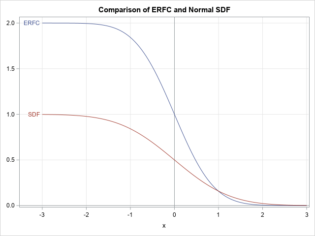
Again, the functions are graphically similar. The range of the ERFC function is [0, 2] whereas the range of the SFD function is [0, 1]. There is the same scaling difference. A little bit of algebra reveals that
SDF(x) = 1/2 ERFC(x/sqrt(2))
If you want, you can modify DATA step in the previous section to verify that these two expressions are equal to within machine precision.

Summary

In summary, the ERF function is used in science and engineering, whereas the normal CDF function is used in probability and statistics. But these functions are computationally equivalent in the sense that you can use affine transformations to convert one function into the other. The complementary functions (ERFC and SDF) are similarly equivalent. In practice, this means that any expression that uses one function (such as the CDF) can be transformed into an equivalent expression that uses the other function (such as ERF).

In closing, I will remark that I used the ERF function for many years in physics and applied math before I became interested in statistics. Nowadays, I use the CDF function almost exclusively because most problems I solve are related to probability and statistics. In addition, the CDF function extends naturally to different scalings (that is, to random variables X ~ N(μ, σ)) and to other probability distributions. What about you? Leave a comment!

Blogs