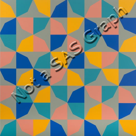
Art evokes an emotional response in the viewer, but sometimes art also evokes a cerebral response. When I see patterns and symmetries in art, I think about a related mathematical object or process. Recently, a Twitter user tweeted about a painting called "Phantom’s Shadow, 2018" by the Nigerian-born artist, Odili Donald Odita. A modified version of the artwork is shown to the right.

The artwork is beautiful, but it also contains a lot of math. The image shows 64 rotations, reflections, and translations of a polygon in four colors. As I will soon explain, the image can also be viewed as 4 x 4 grid where each cell contains a four-bladed pinwheel. The grid displays rotations and reflections of a pinwheel shape.

When I saw this artwork, it inspired me to look closely at its mathematical structure and to create my own mathematical version of the artwork in SAS. This article shows how to use rotations to create a pinwheel from a polygon. A second article discusses how to use rotations and reflections to create a mathematical interpretation of Odita's painting.

Create a polygon

Look closely at the upper left corner of "Phantom's Shadow." You will see the following pinwheel-shaped figure:

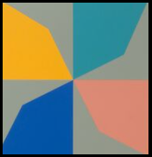
If the center of the pinwheel is the origin, then this pinwheel is based on a sequence of 90-degree rotations of the teal-colored polygon about the origin. Each rotation is a different color (teal, orange, blue, and salmon) on a gray background.

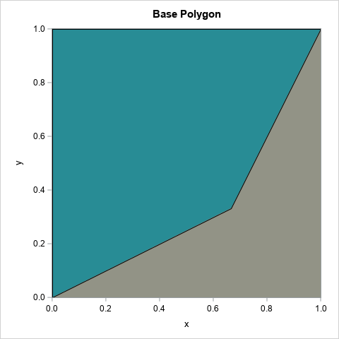
You can assign coordinates to the vertices of the teal polygon. If three vertices are on the corners of the unit square, the fourth vertex appears to be at (2/3, 1/3). You can put the vertices into a SAS data set and graph the polygon by using the POLYGON statement in PROC SGPLOT:

%let alpha = 0.333;          /* Odita's work uses a vertex as (1-alpha, alpha) */
data Poly1;
ID = 1;
input x y @@;
if x=. then do;              /* just for fun, support other locations of vertex */
   x = 1 - α y = α
end;
datalines;
0 0   . .   1 1   0 1   0 0
;
 
%let blue   = CX0f5098;
%let orange = CXeba411;
%let teal   = CX288c95;
%let salmon = CXd5856e;
%let gray   = CX929386;
 
ods graphics / width=480px height=480px;
title "Base Polygon";
proc sgplot data=Poly1 aspect=1;
   styleattrs wallcolor=&gray;
   polygon x=x y=y ID=ID / fill fillattrs=(color=&teal) outline;
   xaxis offsetmin=0.005 offsetmax=0;
   yaxis offsetmin=0 offsetmax=0.005;
run;

The complete artwork repeats this polygon 64 times in a grid by using different colors and different orientations. But the colors and orientations are not random—although that would also look cool! Instead, there is an additional structure. The polygon is part of a pinwheel, and the pinwheel shape is rotated and reflected 16 times in a 4 x 4 grid. The next section shows how to create the pinwheel.

Create a pinwheel

It is possible to perform 2-D rotations and reflections in the DATA step, but the rotations and reflections of a planar figure are most simply expressed in terms of 2 x 2 orthogonal matrices.

To form the pinwheel from the basic polygon, you can use a group of four matrices. All rotations are in the counter-clockwise direction about the origin:

• R₀ is the identity matrix
• R₁ is the matrix that rotates a point 90 degrees (about the origin)
• R₂ is the matrix that rotates a point 180 degrees
• R₃ is the matrix that rotates a point 270 degrees

You do not need advanced mathematics to understand rotations by 90 degrees. However, these four rotation matrices are an example of an algebraic structure called a finite group. These matrices form the cyclic group of order 4 (C₄), where the group operation is matrix multiplication.

Regardless of their name, you can use these matrices to transform the polygon into a pinwheel. The following SAS/IML program reads in the base polygon and transforms it according to each of the four matrices. You can then plot the four images, each in a different color.

/* rotate polygon about the origin to form a pinwheel */
proc iml;
/* actions of the C4 cyclic group: rotations by 90 degrees */
start C4Action(v, act);
   if      act=0 then M = { 1  0,  0  1};
   else if act=1 then M = { 0 -1,  1  0};
   else if act=2 then M = {-1  0,  0 -1};
   else if act=3 then M = { 0  1, -1  0};
   return( v*M` );  /* = (M*z`)` */
finish;
 
use Poly1;  read all var {x y} into P;  close;   /* read the polygon */
 
/* write the pinwheel */
Q = {. . .};
create Shape from Q[c={'ID' 'x' 'y'}];
do i = 0 to 3;
   R = C4Action(P, i);          /* rotated image of polygon     */
   Q = j(nrow(R), 1, i) || R;   /* save the image to a data set */
   append from Q;
end;
close;
QUIT;
 
title "Pinwheel Figure";
title2 "Colors=(Teal, Orange, Blue, Salmon)";
proc sgplot data=Shape aspect=1;
   styleattrs wallcolor=&gray datacolors=(&teal &orange &blue &salmon);
   polygon x=x y=y ID=ID / group=ID fill;
   xaxis offsetmin=0 offsetmax=0;
   yaxis offsetmin=0 offsetmax=0;
run;

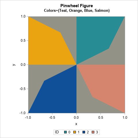
The resulting image is the four-blade pinwheel, which is the basis of Odita's artwork.

A grid of pinwheels

The rest of "Phantom’s Shadow, 2018" can be described in terms of rotations and reflections of the pinwheel shape...with a twist! The next article introduces the dihedral group of order 4 (D4). This is a finite group of order eight and is the symmetry group of the square. It turns out that you can use the elements of D4 to generate the 16 pinwheels in Odita's artwork. You can then use PROC SGPANEL in SAS to generate a graph that looks like "Phantom's Shadow," or you can create your own Odita-inspired mathematical artwork! Stay tuned!