Iterative proportional fitting in SAS

I previously wrote about the RAS algorithm, which is a simple algorithm that performs matrix balancing. Matrix balancing refers to adjusting the cells of a frequency table to match known values of the row and column sums. Ideally, the balanced matrix will reflect the structural relationships in the original matrix. An alternative method is the iterative proportional fitting (IPF) algorithm, which is implemented in the IPF subroutine in SAS/IML. The IPF method can balance n-way tables, n ≥ 2.

The IPF function is a statistical modeling method. It computes maximum likelihood estimates for a hierarchical log-linear model of the counts as a function of the categorical variables. It is more complicated to use than the RAS algorithm, but it is also more powerful.

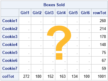
This article shows how to use the IPF subroutine for the two-way frequency table from my previous article. The data are for six girl scouts who sold seven types of cookies. We know the row totals for the Type variable (the boxes sold for each cookie type) and the column totals for the Person variable (the boxes sold by each girl). But we do not know the values of the individual cells, which are the Type-by-Person totals. A matrix balancing algorithm takes any guess for the table and maps it into a table that has the observed row and column sums.

Construct a table that has the observed marginal totals

As mentioned in the previous article, there are an infinite number of matrices that have the observed row and column totals. Before we discuss the IPF algorithm, I want to point out that it is easy to compute one particular balanced matrix. The special matrix is the one that assumes no association (independence) between the Type and Person variables. That matrix is formed by the the outer product of the marginal totals:
B[i,j] = (sum of row i)(sum of col j) / (sum of all counts)

It is simple to compute the "no-association" matrix in the SAS/IML language:

proc iml;
/* Known quantities: row totals and column totals */
u = {260, 214, 178, 148, 75, 67, 59}; /* total boxes sold, by type */
v = {272 180 152 163 134 100};        /* total boxes sold, by girl */
 
/* Compute the INDEPENDENT table, which is formed by the outer product
   of the marginal totals:
   B[i,j] = (sum of row i)(sum of col j) / (sum of all counts) */
B = u*v / sum(u);
 
Type   = 'Cookie1':'Cookie7';                  /* row labels    */
Person = 'Girl1':'Girl6';                      /* column labels */
print B[r=Type c=Person format=7.1 L='Independent Table'];

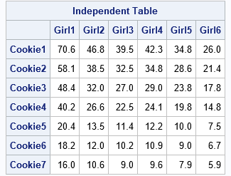
For this balanced matrix, there is no association between the row and column variables (by design). This matrix is the "expected count" matrix that is used in a chi-square test for independence between the Type and Person variables.

Because the cookie types are listed in order from most popular to least popular, the values in the balanced matrix (B) decrease down each column. If you order the girls according to how many boxes they sold (you need to exchange the third and fourth columns), then the values in the balanced matrix would decrease across each row.

Use the IPF routine to balance a matrix

The documentation for the IPF subroutine states that you need to specify the following input arguments. For clarity, I will only discuss two-way r x c tables.

dim: The vector of dimensions of the table: dim = {r c};
table: This r x c matrix is used to specify the row and column totals. You can specify any matrix; only the marginal totals of the matrix are used. For example, for a two-way table, you can use the "no association" matrix from the previous section.
config is an input matrix whose columns specify which marginal totals to use to fit the counts. Because the model is hierarchical, all subsets of specified marginals are included in the model. For a two-way table, the most common choices are the main effect models such as config={1} (model count by first variable only), config={2} (model count by second variable only), and config={1 2} (model count by using both variables). It is possible to fit the "fully saturated model" (config={1, 2}), but that model is overparameterized and results in a perfect fit, if the IPF algorithm converges.
initTable (optional): The elements of this matrix will be adjusted to match the observed marginal totals. In practice, this matrix is often based on a survey and you want to adjust the counts by using known marginal totals from a recent census of the population. Or it might be an educated guess, as in the Girl Scout cookie example. If you do not specify this matrix, a matrix of all 1s is used, which implies that you think all cell entries are approximately equal.

The following SAS/IML program defines the parameters for the IPF call.

/* Specify structure between rows and columns by asking each girl 
   to estimate how many boxes of each type she sold. This is the 
   matrix whose cells will be adjusted to match the marginal totals. */
/*   G1 G2 G3 G4 G5 G6          */
A = {75 45 40 40 40 30 ,  /* C1 */
     40 35 45 35 30 30 ,  /* C2 */
     40 25 30 40 30 20 ,  /* C3 */
     40 25 25 20 20 20 ,  /* C4 */
     30 25  0 10 10  0 ,  /* C5 */
     20 10 10 10 10  0 ,  /* C6 */
     20 10  0 10  0  0 }; /* C7 */
 
Dim = ncol(A) || nrow(A);  /* dimensions of r x c table */
Config = {1 2};            /* model main effects: counts depend on Person and Type */
call IPF(FitA, Status,     /* output values */
         Dim, B,           /* use the "no association" matrix to specify marginals */
         Config, A);       /* use best-guess matrix to specify structure */
print FitA[r=Type c=Person format=7.2],     /* the IPF call returns the FitA matrix and Status vector */
      Status[c={'rc' 'Max Diff' 'Iters'}];

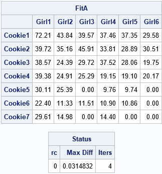
The IPF call returns two quantities. The first output is the balanced matrix. For this example, the balanced matrix (FitA) is identical to the result from the RAS algorithm. It has a similar structure to the "best guess" matrix (A). For example, and notice that the cells in the original matrix that are zero are also zero in the balanced matrix.

The second output is the Status vector. The status vector provides information about the convergence of the IPF algorithm:

If the first element is zero, the IPF algorithm converged.
The second element gives the maximum difference between the marginal totals of the balanced matrix (FitA) and the observed marginal totals.
The third element gives the number of iterations of the IPF algorithm.

Other models

The IPF subroutine is more powerful than the RAS algorithm because you can fit n-way tables and because you can model the table in several natural ways. For example, the model in the previous section assumes that the counts depend on the salesgirl and on the cookie type. You can also model the situation where the counts depend only on one of the factors and not on the other:

/* counts depend only on Person, not on cookie Type */
Config = {1};   
call IPF(FitA1, Status, Dim, B, Config, A);
print FitA1[r=Type c=Person format=7.2], Status;
 
/* counts depend only on cookie Type, not on Person */
Config = {2};   
call IPF(FitA2, Status, Dim, B, Config, A);
print FitA2[r=Type c=Person format=7.2], Status;

Summary

In summary, the SAS/IML language provides a built-in function (CALL IPF) for matrix balancing of frequency tables. The routine incorporates statistical modeling and you can specify which variables to use to model the cell counts. The documentation several examples that demonstrate using the IPF algorthm to balance n-way tables, n ≥ 2.

Blogs