I recently read an article that describes ways to compute confidence intervals for the difference in a percentile between two groups. In Eaton, Moore, and MacKenzie (2019), the authors describe a problem in hydrology. The data are the sizes of pebbles (grains) in rivers at two different sites. The authors ask whether the p_th percentile of size is significantly different between the two sites. They also want a confidence interval for the difference. The median (50th percentile) and 84th percentile were the main focus of their paper.

For those of us who are not hydrologists, consider a sample from group 'A' and a sample from group 'B'. The problem is to test whether the p_th percentile is different in the two groups and to construct a confidence interval for the difference.

The authors show two methods: a binomial-based probability model (Section 2) and a bootstrap confidence interval (Section 3). However, there is another option: use quantile regression to estimate the difference in the quantiles and to construct a confidence interval. In this article, I show the computation for the 50th and 84th percentiles and compare the results to a bootstrap estimate. You can download the SAS program that creates the analyses and graphs in this article.

If you are not familiar with quantile regression, see my previous article about how to use quantile regression to estimate the difference between two medians.

A data distribution of particle sizes

For convenience, I simulated samples for the sizes of pebbles in two stream beds:

• For Site 'A', the sizes are lognormally distributed with μ=0.64 and σ=1. For the LN(0.64, 1) distribution, the median pebble size is 1.9 mm and the size for the 84th percentile is 5.1 mm.
• For Site 'B', the sizes are lognormally distributed with μ=0.53 and σ=1. For the LN(0.53, 1) distribution, the median pebble size is 1.7 mm and the size for the 84th percentile is 4.6 mm.

I assume that sizes are measured to the nearest 0.1 mm. I simulated 500 pebbles from Site 'A' and 300 pebbles from Site 'B'. You can use PROC UNIVARIATE in SAS to compute a comparative histogram and to compute the percentiles. The sample distributions are shown below:

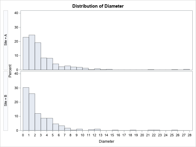
For Site 'A', the estimates for the sample median and 84th percentile are 2.05 mm and 5.1 mm, respectively. For Site 'B', the estimates are 1.60 mm and 4.7 mm, respectively. These estimates are close to their respective parameter values.

Estimate difference in percentiles

The QUANTREG procedure in SAS makes it easy to estimate the difference in the 50th and 84th percentiles between the two groups. The syntax for the QUANTREG procedure is similar to other SAS regression procedures such as PROC GLM:

proc quantreg data=Grains;
   class Site;
   model Diameter = Site / quantile=0.5 0.84;
   estimate 'Diff in Pctl' Site 1 -1 / CL;
run;

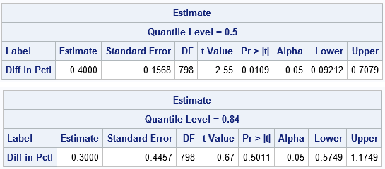
The output from PROC QUANTREG shows estimates for the difference between the percentiles of the two groups. For the 50th percentile, an estimate for the difference is 0.4 with a 95% confidence of [0.09, 0.71]. Because 0 is not in the confidence interval, you can conclude that the median pebble size at Site 'A' is significantly different from the median pebble size at Site 'B'. For the 84th percentile, an estimate for the difference is 0.3 with a 95% confidence of [-0.57, 1.17]. Because 0 is in the interval, the difference between the 84th percentiles is not significantly different from 0.

Methods for estimating confidence intervals

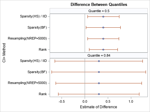
The QUANTREG procedure supports several different methods for estimating a confidence interval: sparsity, rank, and resampling. The estimates in the previous section are by using the RANK method, which is the default for smaller data sets. You can use the CI= option on the PROC QUANTREG statement to use these methods and to specify options for the methods. The following graph summarizes the results for four combinations of methods and options. The results of the analysis do not change: The medians are significantly different but the 84th percentiles are not.

A comparison with bootstrap estimates

When you use a resampling-based estimate for the confidence interval, the interval depends on the random number seed, the algorithm used to generate random numbers, and the number of bootstrap iterations. This can make it hard to compare Monte Carlo results to the results from deterministic statistical methods. Nevertheless, I will present one result from a bootstrap analysis of the simulated data. The following table shows the bootstrap percentile estimates (used by Eaton, Moore, and MacKenzie (2019)) for the difference between percentiles.

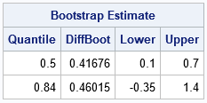
The confidence intervals (the Lower and Upper columns of the table) are comparable to the intervals produced by PROC QUANTREG. The confidence interval for the difference between medians seems equivalent. The bootstrap interval for the 84th percentile is shifted to the right relative to the QUANTREG intervals. However, the inferences are the same: the medians are different but there is no significant difference between the 84th percentiles.

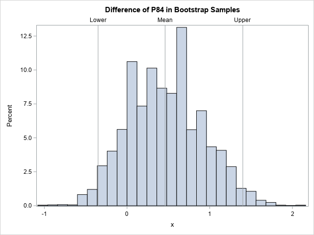
The following histogram shows the difference between the 84th percentiles for 5,000 bootstrap samples. The confidence interval is determined by the 2.5th and 97.5th percentiles of the bootstrap distribution. The computation requires only a short SAS/IML program, which runs very quickly.

Summary

Data analysts might struggle to find an easy way to compute the difference between percentiles for two (or more) groups. A recent paper by Eaton, Moore, and MacKenzie (2019) proposes one solution, which is to use resampling methods. An alternative is to use quantile regression to estimate the difference between percentiles, as shown in this article. I demonstrate the method by using simulated data of the form studied by Eaton, Moore, and MacKenzie.

You can download the SAS program that creates the analyses and graphs in this article.