I have written several articles about how to work with continuous probability distributions in SAS. I always emphasize that it is important to be able to compute the four essential functions for working with a statistical distribution. Namely, you need to know how to generate random values, how to compute the PDF, how to compute the CDF, and how to compute quantiles. In this article, I describe how to compute each of the four quantities for the geometric distribution, which is a DISCRETE probability distribution. The graphs that visualize a discrete distribution are slightly different than for continuous distributions. Also, the geometric distribution has two different definitions, and I show how to work with either definition in SAS.

The definition of the geometric distribution

A Bernoulli trial is an experiment that has two results, usually referred to as a "failure" or a "success." The success occurs with probability p and the failure occurs with probability 1-p. "Success" means that a specific event occurred whereas "failure" indicates that the event did not occur. Because the event can be negative (death, recurrence of cancer, ...) sometimes a "success" is not a cause for celebration!

The geometric distribution has two definitions:

1. The number of trials until the first success in a sequence of independent Bernoulli trials. The possible values are 1, 2, 3, ....
2. The number of failures before the first success in a sequence of independent Bernoulli trials. The possible values are 0, 1, 2, ....

Obviously, the two definitions are closely related. If X is a geometric random variable according to the first definition, then Y=X-1 is a geometric random variable according to the second definition. For example, define "heads" as the event that you want to monitor. If you toss a coin and it first shows heads on the third toss, then the number of trials until the first success is 3 and the number of failures is 2. Whenever you work with the geometric distribution (or its generalization, the negative binomial distribution), you should check to see which definition is being used.

The definition of the geometric distribution in SAS software

It is regrettable that SAS was not consistent in choosing a definition. The first definition is used by the RAND function to generate random variates. The second definition is used by the PDF function, the CDF function, and the QUANTILE function. In this article, I will use the "number of trials," which is the first definition. In my experience, this definition is more useful in applications. I will point out how to adjust the syntax of the SAS functions so that they work for either definition.

The probability mass function for the geometric distribution

For a discrete probability distribution, the probability mass function (PMF) gives the probability of each possible value of the random variable. So for the geometric distribution, we want to compute and visualize the probabilities for n=1, 2, 3,... trials.

The probabilities depend on the parameter p, which is the probability of success. I will use three different values to illustrate how the geometric distribution depends on the parameter:

• p = 1/2 = 0.5: the probability of "heads" when you toss a coin
• p = 1/6 = 0.166: the probability of rolling a 6 with a six-sided die
• p = 1/13 = 0.077: the probability of drawing an ace from a shuffled deck of 52 cards

The following SAS DATA step uses the PDF function to compute the probabilities for these three cases. The parameters in the PDF function are the number of failures and the probability of success. If you let n be the number of trials until success, then n-1 is the number of failures before success. Thus, the following statements use n-1 as a parameter. Since I will need the cumulative probabilities in the next section, I use the CDF function to compute them in the same DATA step:

data Geometric;
do p = 0.5, 0.166, 0.077;
   /* We want the probability that the event occurs on the n_th trial.
      This is the same as the probability of n-1 failure before the event. */
   do n = 1 to 16;                     
      pdf = pdf("Geometric", n-1, p);  /* probability that event occurs on the n_th trial */
      cdf = cdf("Geometric", n-1, p);  /* probability that event happens on or before n_th Trial*/
      output;
   end;
end;
run;
 
title "Probability Mass Function for Geom(p)";
proc sgplot data=Geometric;
   scatter x=n y=pdf / group=p markerattrs=(symbol=CircleFilled);
   series  x=n y=pdf / group=p lineattrs=(color=Gray);
   label n="Number of Trials" pdf="Probability of Event";
   xaxis grid integer values=(0 to 16 by 2) valueshint;
run;

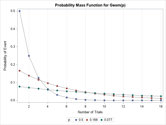
If you are visualizing the PMF for one value of p, I suggest that you use a bar chart. Because I am showing multiple PMFs in one graph, I decided to use a scatter plot to indicate the probabilities, and I used gray lines to visually connect the probabilities that belong to the same distribution. This is the same technique that is used on the Wikipedia page for the geometric distribution.

For large probabilities, the PMF probability decreases rapidly. When the probability for success is large, the event usually occurs early; it is rare that you would have to wait for many trials before the event occurs. This geometric rate of decrease is why the distribution is named the "geometric" distribution! For small probabilities, the PMF probability decreases slowly. It is common to wait for many trials before the first success occurs.

The cumulative probability function

If you want to know the cumulative probability that the event occurs on or before the nth trial, you can use the CDF function. The CDF curve was computed in the previous section for all three probabilities. The following call to PROC SGPLOT creates a graph. If I were plotting a single distribution, I would use a bar chart. Because I am plotting several distributions, the call uses the STEP statement to create a step plot for the discrete horizontal axis. However, if you want to show the CDF for many trials (maybe 100 or more), then you can use the SERIES statement because at that scale the curve will look smooth to the eye.

title "Cumulative Distribution for Geom(p)";
title2 "Probability That Event Occurs on or before n_th Trial";
proc sgplot data=Geometric;
   step x=n y=cdf / group=p curvelabel markers markerattrs=(symbol=CircleFilled);
   label n="Number of Trials" cdf="Cumulative Probability";
   xaxis grid integer values=(0 to 16 by 2) valueshint;
   yaxis grid;
run;

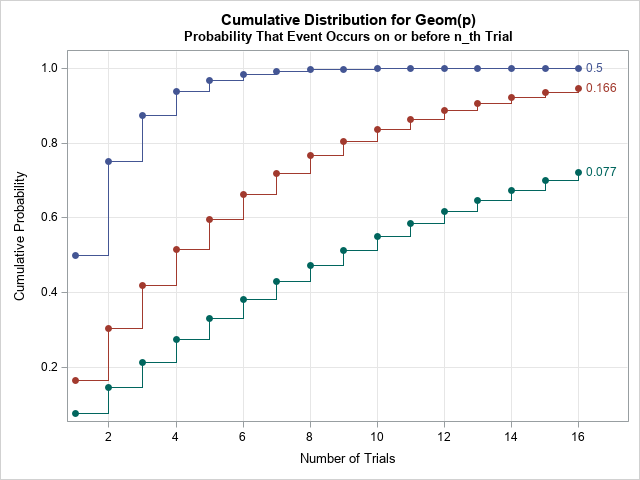
The cumulative probability increases quickly when the probability of the event is high. When the probability is low, the cumulative probability is initially almost linear. You can prove this by using a Taylor series expansion of the CDF, as follows. The formula for the CDF is F(n) = 1 – (1 – p)ⁿ. When p is much much less than 1 (written p ≪ 1), then (1 – p)ⁿ ≈ 1 – n p + .... Consequently, the CDF is nearly linear (with slope p) as a function of n when p ≪ 1.

Quantiles of the geometric distribution

When the density function (PDF) of a continuous distribution is positive, the CDF is strictly increasing. Consequently, the inverse CDF function is continuous and increasing. For discrete distributions, the CDF function is a step function, and the quantile is the smallest value for which the CDF is greater than or equal to the given probability. Consequently, the quantile function is also a step function. The following DATA step uses the QUANTILE function to compute the quantiles for p=1/6 and for evenly spaced values of the cumulative probability.

data Quantile;
prob = 0.166;
do p = 0.01 to 0.99 by 0.005;
   n = quantile("Geometric", p, prob); * number of failures until event;
   n = n+1;                            * number of trials until event;
   output;
end;
run;
 
title "Quantiles for Geom(0.166)";
proc sgplot data=Quantile;
   scatter x=p y=n / markerattrs=(symbol=CircleFilled);
   label n="Number of Trials" p="Cumulative Probability";
   xaxis grid;
   yaxis grid;
run;

Random variates

For a discrete distribution, it is common to use a bar chart to show a random sample. For a large sample, you might choose a histogram. However, I think it is useful to plot the individual values in the sample, especially if some of the random variates are extreme values. You can Imagine 20 students who each roll a six-side die until it shows 6. The following DATA step simulates this experiment.

%let numSamples = 20;           *sample of 20 people;
data RandGeom;
call streaminit(12345);         * random seed for covid-19;
p = 0.166;                      * 1/6 ~ 0.166;
do ID = 1 to &numSamples;
   x = rand("Geometric", p);    *number of trials until event occurs;
   /* if you want the number of failures before the event: x = x-1 */
   Zero = 0;
   output;
end;
run;

In the simulated random sample, the values range from 1 (got a 6 on the first roll) to 26 (waited a long time before a 6 appeared). You can create a bar chart that shows these values. You can also add reference lines to the chart to indicate the mean and median of the Geom(1/6) distribution. For a Geom(p) distribution, the expected value is 1/p and the median of the distribution is ceil( -1/log₂(1-p) ). When p = 1/6, the expected value is 6 and the median value is 4.

When a bar chart contains a few very long bars, you might want to "clip" the bars at some reference value so that the smaller bars are visible. The HIGHLOW statement in PROC SGPLOT supports the CLIPCAP option, which truncates the bar and places an arrow to indicate that the true length of the bar is longer than indicated in the graph. If you add labels to the end of each bar, the reader can see the true value even though the bar is truncated in length, as follows:

proc sort data=RandGeom;
   by x;
run;
/* compute mean and median of the Geom(1/6) distribution */
data Stats;
p = 0.166;
PopMean = 1/p;                    PopMedian = ceil( -1/log2(1-p) );
call symputx("PopMean", PopMean); call symputx("PopMedian", PopMedian);
run;
 
/* use CLIPCAP amd MAX= option to prevent long bars */
title "&numSamples Random Rolls of a Six-side Die";
title2 "Random Sample of Geom(0.166)";
proc sgplot data=RandGeom;
   highlow y=ID low=Zero high=x / type=bar highlabel=x    CLIPCAP; 
   refline &PopMean / axis=x label="Mean" labelpos=min; 
   refline &PopMedian / axis=x label="Population Median" labelpos=min; 
   xaxis grid label="Number of Trials until Event" minor  MAX=10;  
   yaxis type=discrete discreteorder=data reverse valueattrs=(size=7);
run;

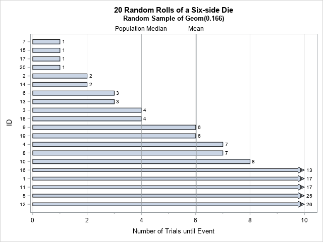
This chart shows that four students got "lucky" and observed a 6 on their first roll. Half the students observed a 6 is four or fewer rolls, which is the median value of the Geom(1/6) distribution. Some students rolled many times before seeing a 6. The graph is truncated at 10, and students who required more than 10 rolls are indicated by an arrow.

Conclusions

This article shows how to compute the four essential functions for the geometric distribution. The geometric distribution is a discrete probability distribution. Consequently, some concepts are different than for continuous distributions. SAS provides functions for the PMF, CDF, quantiles, and random variates. However, you need to be careful because there are two common ways to define the geometric distribution. The SAS statements in this article show how to define the geometric distribution as the number of trials until an event occurs. However, with minor modifications, the same program can handle the second definition, which is the number of failures before the event.

The geometric distribution is a simple model for many random events such as tossing coins, rolling dice, and drawing cards. Although it is too simple for many real-world phenomena, it demonstrates how the cumulative probability of an event depends on the number of trials and the probability of the event. For example, you can use the geometric model to explain why social distancing and disinfecting surfaces can reduce the spread of a viral disease.

You can download the complete SAS code that generates the graphs in this article.