Recently someone on social media asked, "how can I compute the required sample size for a binomial test?" I assume from the question that the researcher was designing an experiment to test the proportions between two groups, such as a control group and a treatment/intervention group. They wanted to know how big they should make each group.

It's a great question, and it highlights one of the differences between statistics and machine learning. Statistics does not merely analyze data after they are collected. It also helps you to design experiments. Without statistics, a researcher might assign some number of subjects to each treatment group, cross his fingers for luck, and hope that the difference between the groups will be significant. With statistics, you can determine in advance how many subjects you need to detect a specified difference between the groups. This can save time and money: having too many subjects is needlessly expensive; having too few does not provide enough data to confidently answer the research question. To estimate the group size, you must have some prior knowledge (or estimate) of the size of the effect you are trying to measure. You can use smaller groups if you are trying to detect a large effect; you need larger groups to detect a small effect.

Researchers use power and sample size computations to address these issues. "Sample size" is self-explanatory. "Power" is the probability that a statistical test will reject the null hypothesis when the alternative hypothesis is true. In general, the power of a test increases with the sample size. More power means fewer Type II errors (fewer "false negatives").

In SAS, there are several ways to perform computations related to power and sample size, but the one that provides information about binomial proportions is PROC POWER. This article shows how to use PROC POWER to determine the sample size that you need for a binomial test for proportions in two independent samples.

Sample size to detect difference in proportion

Many US states have end-of-course (EOC) assessments, which help school administrators measure how well students are mastering fundamental topics such as reading and math. I read about a certain school district in which only 31% of high school students are passing the algebra EOC assessment. Suppose a company wants to sell the district software that it claims will boost student passing by two percentage points (to 33%). The administrators are interested, but the software is expensive, so they decide to conduct a pilot study to investigate the company's claim. How big must the study be?

The researchers need to calculate how many students are needed to detect a difference in the proportion of 2% (0.02). Before we do any calculations, what does your intuition say? Would 100 students in each group be enough? Would 500 students be enough? The TWOSAMPLEFREQ statement in the POWER procedure in SAS can help answer that question.

PROC POWER and a one-sided test for proportion

The POWER procedure can compute power and sample size for more than a dozen common statistical tests. In addition, you can specify multiple estimates of the parameters in the problem (for example, the true proportions) to see how sensitive the results are to your assumptions. You can also specify whether to perform a two-sided test (the default), a one-sided test, or tests for superiority or inferiority. (For information about inferiority and superiority testing, see Castelloe and Watts (2015).)

Let's analyze the results by using a one-tailed chi-square test for the difference between two proportions (from independent samples). The null hypothesis is that the control group and the "Software" group each pass the EOC test 31% of the time. The alternative hypothesis is that a higher proportion of the software group passes the test.

You can use the TWOSAMPLEFREQ statement in the POWER procedure to determine the sample sizes required to give 80% power to detect a proportion difference of at least 0.02. You use a missing value (.) to specify the parameter that the procedure should solve for, which in this case is the number of subjects in each treatment group (NPERGROUP). The GROUPPROPORTIONS= option specifies the hypothesized proportions, or you can use the REFPROPORTION= and PROPORTIONDIFF= options. The following call to PROC POWER solves for the sample size in a balanced experiment with two groups:

proc power; 
  twosamplefreq test=FM
  groupproportions = (0.31  0.33) /* OR: refproportion=0.31 proportiondiff=0.02 */
  power = 0.8
  alpha = 0.05
  npergroup = . 
  sides = 1;
run;

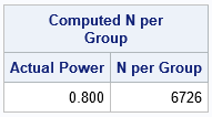
The output indicates that the school district needs 6,726 students in each group in order to verify the company's claims with 80% power! I was surprised by this number, which is much bigger than my intuition suggested!

The power for various sample sizes

What if I hadn't used PROC POWER? What if I had just assigned 1,000 to each group? Or 2,000 students? What power would the test of proportions have to detect the small difference of proportion (0.02), if it exists? PROC POWER can answer that question, too. It turns out that a sample size of N=1000 only results in 0.25 power and a sample size of N=2000 only results in a power of 0.39. A pilot study based on those smaller samples is a waste of time and money because the study isn't large enough to detect the small effect that the company claims.

PROC POWER makes it easy to create a graph that plots the power of the binomial test for proportions against the sample size for a range of samples. You can also display the power for a range of sample sizes, as follows:

proc power; 
  twosamplefreq test=pchi
  refproportion = 0.31 proportiondiff = 0.02
  power = .
  alpha = 0.05
  npergroup = 250 to 8000 by 250 
  sides = 1;
  plot x=n xopts=(ref=1000 2000 5000 6726 crossref=yes);
  ods exclude output;
run;

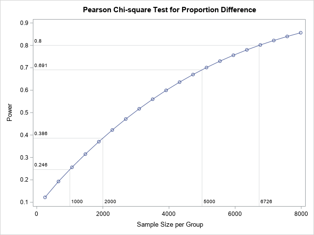
The graph shows that samples that have 1,000 or even 2,000 students in each group do not have enough power to detect a small difference of proportion (0.02) with any confidence. Only for N ≥ 5,000 does the power of the test start to approach reasonable levels.

Quick check: Simulate a sample

Whenever I see a counterintuitive result, I like to run a quick simulation to see whether the simulation agrees with the analysis. The following program generates a random sample from two groups of size N=1,000. The control group has a 31% chance of passing the test; the "Software" group has a 33% chance. A PROC FREQ analysis for the difference in proportions indicates that the empirical difference between the groups is about 0.02, but the p-value for the one-sided test is 0.18, which does not enable you to conclude that there is a significant difference between the proportions of the two groups.

/* simulation of power */
%let N = 1000;             /* group sizes*/
%let p = 0.31;             /* reference proportion */
%let delta = 0.02;         /* true size of difference in proportions */
 
data PowerSim(drop=i);
call streaminit(321);
do i = 1 to &N;
   c='Control '; pass = rand("Bernoulli", &p);        output; /* x ~ Bern(p) */
   c='Software'; pass = rand("Bernoulli", &p+&Delta); output; /* x ~ Bern(p+delta) */
end;
run;
 
proc freq data=PowerSim;
tables c*pass / chisq riskdiff(equal var=null cl=wald) /* Wald test for equality of proportions */
             nocum norow nopct nocol;
run;

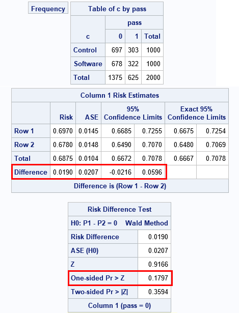
Part of the output from PROC FREQ is shown. The output displays a typical two-way frequency table for the simulated experiment. You can see that the raw number of students that pass/fail the test are very similar. In healthcare applications, binomial proportions often correspond to "risks," so a "risk difference" is a difference in proportions. The RISKDIFF option tests whether the difference of proportions (risks) is zero. The output from the test shows both the two-sided and one-sided results. For these simulated data, there is insufficient evidence to reject the null hypothesis of no difference.

If you change the value of the macro variable N to a larger number (such as N = 6,726), it is increasingly likely that the chi-square test will be able to conclude that there is a significant difference between the proportions. In fact, for N = 6,726, you would expect 80% of the simulated samples to correctly reject the null hypothesis. Simulation is a way to create a power-by-sample-size curve even when there is not an explicit formula that relates the two quantities.

In summary, the statistical concepts of power and sample size can help researchers plan their experiments. This is a powerful idea! (Pun intended!) It can help you know in advance how large your samples should be when you need to detect a small effect.