Biplots are two-dimensional plots that help to visualize relationships in high dimensional data. A previous article discusses how to interpret biplots for continuous variables. The biplot projects observations and variables onto the span of the first two principal components. The observations are plotted as markers; the variables are plotted as vectors. The observations and/or vectors are not usually on the same scale, so they need to be rescaled so that they fit on the same plot. There are four common scalings (GH, COV, JK, and SYM), which are discussed in the previous article.

This article shows how to create biplots in SAS. In particular, the goal is to create the biplots by using modern ODS statistical graphics. You can obtain biplots that use the traditional SAS/GRAPH system by using the %BIPLOT macro by Michael Friendly. The %BIPLOT macro is very powerful and flexible; it is discussed later in this article.

There are four ways to create biplots in SAS by using ODS statistical graphics:

• You can use PROC PRINQUAL in SAS/STAT software to create the COV biplot.
• If you have a license for SAS/GRAPH software (and SAS/IML software), you can use Friendly's %BIPLOT macro and use the OUT= option in the macro to save the coordinates of the markers and vectors. You can then use PROC SGPLOT to create a modern version of Friendly's biplot.
• You can use the matrix computations in SAS/IML to "manually" compute the coordinates of the markers and vectors. (These same computations are performed internally by the %BIPLOT macro.) You can use the Biplot module to create a biplot. Alternatively, you can use the WriteBiplot module to create a SAS data set that contains the biplot coordinates and use PROC SGPLOT to create the biplot.

For consistency with the previous article, all methods in this article standardize the input variables to have mean zero and unit variance (use the SCALE=STD option in the %BIPLOT macro). All biplots show projections of the same four-dimensional Fisher's iris data. The following DATA step assigns a blank label. If you do not supply an ID variable, some biplots display observations numbers.

data iris;
   set Sashelp.iris;
   id = " ";        /* create an empty label variable */
run;

Use PROC PRINQUAL to compute the COV biplot

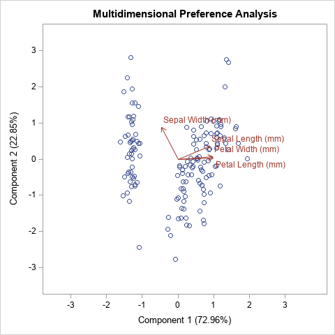
The PRINQUAL procedure can perform a multidimensional preference analysis, which is visualized by using a MDPREF plot. The MDPREF plot is closely related to biplot (Jackson (1991), A User’s Guide to Principal Components, p. 204). You can get PROC PRINQUAL to produce a COV biplot by doing the following:

• Use the N=2 option to specify you want to compute two principal components.
• Use the MDPREF=1 option to specify that the procedure should not rescale the vectors in the biplot. By default, MDPREF=2.5 and the vectors appear 2.5 larger than they should be. (More on scaling vectors later.)
• Use the IDENTITY transformation so that the variables are not transformed in a nonlinear manner.

The following PROC PRINQUAL statements produce a COV biplot (click to enlarge):

proc prinqual data=iris plots=(MDPref) 
              n=2       /* project onto Prin1 and Prin2 */
              mdpref=1; /* use COV scaling */
   transform identity(SepalLength SepalWidth PetalLength PetalWidth);  /* identity transform */
   id ID;
   ods select MDPrefPlot;
run;

Use Friendly's %BIPLOT macro

Friendly's books [SAS System for Statistical Graphics (1991) and Visualizing Categorical Data (2000)] introduced many SAS data analysts to the power of using visualization to accompany statistical analysis, and especially the analysis of multivariate data. His macros use traditional SAS/GRAPH graphics from the 1990s. In the mid-2000s, SAS introduced ODS statistical graphics, which were released with SAS 9.2. Although the %BIPLOT macro does not use ODS statistical graphics directly, the macro supports the OUT= option, which enables you to create an output data set that contains all the coordinates for creating a biplot.

The following example assumes that you have downloaded the %BIPLOT macro and the %EQUATE macro from Michael Friendly's web site.

/* A. Use %BIPLOT macro, which uses SAS/IML to compute the biplot coordinates. 
      Use the OUT= option to get the coordinates for the markers and vectors.
   B. Transpose the data from long to wide form.
   C. Use PROC SGPLOT to create the biplot
*/
%let FACTYPE = SYM;   /* options are GH, COV, JK, SYM */
title "Biplot: &FACTYPE, STD";
%biplot(data=iris, 
        var=SepalLength SepalWidth PetalLength PetalWidth, 
        id=id,
        factype=&FACTYPE,  /* GH, COV, JK, SYM */
        std=std,           /* NONE, MEAN, STD  */
        scale=1,           /* if you do not specify SCALE=1, vectors are auto-scaled */
        out=biplotFriendly,/* write SAS data set with results */ 
        symbols=circle dot, inc=1);
 
/* transpose from long to wide */
data Biplot;
set biplotFriendly(where=(_TYPE_='OBS') rename=(dim1=Prin1 dim2=Prin2 _Name_=_ID_))
    biplotFriendly(where=(_TYPE_='VAR') rename=(dim1=vx dim2=vy _Name_=_Variable_));
run;
 
proc sgplot data=Biplot aspect=1 noautolegend;
   refline 0 / axis=x; refline 0 / axis=y;
   scatter x=Prin1 y=Prin2 / datalabel=_ID_;
   vector  x=vx    y=vy    / datalabel=_Variable_
                             lineattrs=GraphData2 datalabelattrs=GraphData2;
   xaxis grid offsetmin=0.1 offsetmax=0.2;
   yaxis grid;
run;

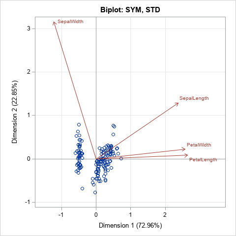
Because you are using PROC SGPLOT to display the biplot, you can easily configure the graph. For example, I added grid lines, which are not part of the output from the %BIPLOT macro. You could easily change attributes such as the size of the fonts or add additional features such as an inset. With a little more work, you can merge the original data and the biplot data and color-code the markers by a grouping variable (such as Species) or by a continuous response variable.

Notice that the %BIPLOT macro supports a SCALE= option. The SCALE= option applies an additional linear scaling to the vectors. You can use this option to increase or decrease the lengths of the vectors in the biplot. For example, in the SYM biplot, shown above, the vectors are long relative to the range of the data. If you want to display vectors that are only 25% as long, you can specify SCALE=0.25. You can specify numbers greater than 1 to increase the vector lengths. For example, SCALE=2 will double the lengths of the vectors. If you omit the SCALE= option or set SCALE=0, then the %BIPLOT macro automatically scales the vectors to the range of the data. If you use the SCALE= option, you should tell the reader that you did so.

SAS/IML modules that compute biplots

The %BIPLOT macro uses SAS/IML software to compute the locations of the markers and vectors for each type of biplot. I wrote three SAS/IML modules that perform the three steps of creating a biplot:

• The CalcBiplot module computes the projections of the observations and scores onto the first few principal components. This module (formerly named CalcPrinCompBiplot) was written in the mid-2000s and has been distributed as part of the SAS/IML Studio application. It returns the scores and vectors as SAS/IML matrices.
• The WriteBiplot module calls the CalcBiplot module and then writes the scores to a SAS data set called _SCORES and the vectors (loadings) to a SAS data set called _VECTORS. It also creates two macro variables, MinAxis and MaxAxis, which you can use if you want to equate the horizontal and vertical scales of the biplot axes.
• The Biplot function calls the WriteBiplot module and then calls PROC SGPLOT to create a biplot. It is the "raw SAS/IML" version of the %BIPLOT macro.

You can use the CalcBiplot module to compute the scores and vectors and return them in IML matrices. You can use the WriteBiplot module if you want that information in SAS data sets so that you can create your own custom biplot. You can use the Biplot module to create standard biplots. The Biplot and WriteBiplot modules are demonstrated in the next sections.

Use the Biplot module in SAS/IML

The syntax of the Biplot module is similar to the %BIPLOT macro for most arguments. The input arguments are as follows:

• X: The numerical data matrix
• ID: A character vector of values used to label rows of X. If you pass in an empty matrix, observation numbers are used to label the markers. This argument is ignored if labelPoints=0.
• varNames: A character vector that contains the names of the columns of X.
• FacType: The type of biplot: 'GH', 'COV', 'JK', or 'SYM'.
• StdMethod: How the original variables are scaled: 'None', 'Mean', or 'Std'.
• Scale: A numerical scalar that specifies additional scaling applied to vectors. By default, SCALE=1, which means the vectors are not scaled. To shrink the vectors, specify a value less than 1. To lengthen the vectors, specify a value greater than 1. (Note: The %BIPLOT macro uses SCALE=0 as its default.)
• labelPoints: A binary 0/1 value. If 0 (the default) points are not labeled. If 1, points are labeled by the ID values. (Note: The %BIPLOT macro always labels points.)

The last two arguments are optional. You can specify them as keyword-value pairs outside of the parentheses. The following examples show how you can call the Biplot module in a SAS/IML program to create a biplot:

ods graphics / width=480px height=480px;
proc iml;
/* assumes the modules have been previously stored */
load module=(CalcBiplot WriteBiplot Biplot);
use sashelp.iris;
read all var _NUM_ into X[rowname=Species colname=varNames];
close;
 
title "COV Biplot with Scaled Vectors and Labels";
run Biplot(X, Species, varNames, "COV", "Std") labelPoints=1;   /* label obs */
 
title "JK Biplot: Relationships between Observations";
run Biplot(X, NULL, varNames, "JK", "Std");
 
title "JK Biplot: Automatic Scaling of Vectors";
run Biplot(X, NULL, varNames, "JK", "Std") scale=0;            /* auto scale; empty ID var */
 
title "SYM Biplot: Vectors Scaled by 0.25";
run Biplot(X, NULL, varNames, "SYM", "Std") scale=0.25;        /* scale vectors by 0.25 */

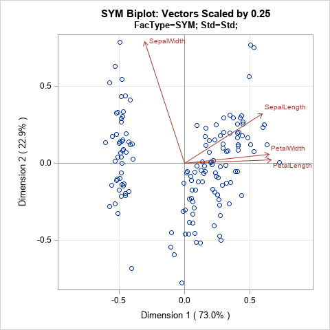
The program creates four biplots, but only the last one is shown. The last plot uses the SCALE=0.25 option to rescale the vectors of the SYM biplot. You can compare this biplot to the SYM biplot in the previous section, which did not rescale the length of the vectors.

Use the WriteBiplot module in SAS/IML

If you prefer to write an output data set and then create the biplot yourself, use the WriteBiplot module. After loading the modules and the data (see the previous section), you can write the biplot coordinates to the _Scores and _Vectors data sets, as follows. A simple DATA step appends the two data sets into a form that is easy to graph:

run WriteBiplot(X, NULL, varNames, "JK", "Std") scale=0;   /* auto scale vectors */
QUIT;
 
data Biplot;
   set _Scores _Vectors;    /* append the two data sets created by the WriteBiplot module */
run;
 
title "JK Biplot: Automatic Scaling of Vectors";
title2 "FacType=JK; Std=Std";
proc sgplot data=Biplot aspect=1 noautolegend;
   refline 0 / axis=x; refline 0 / axis=y;
   scatter x=Prin1 y=Prin2 / ; 
   vector  x=vx    y=vy    / datalabel=_Variable_
                             lineattrs=GraphData2 datalabelattrs=GraphData2;
   xaxis grid offsetmin=0.1 offsetmax=0.1 min=&minAxis max=&maxAxis;
   yaxis grid min=&minAxis max=&maxAxis;
run;

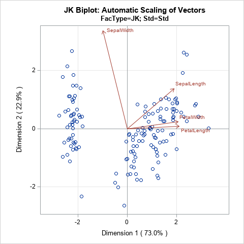
In the program that accompanies this article, there is an additional example in which the biplot data is merged with the original data so that you can color-code the observations by using the Species variable.

Summary

This article shows four ways to use modern ODS statistical graphics to create a biplot in SAS. You can create a COV biplot by using the PRINQUAL procedure. If you have a license for SAS/IML and SAS/GRAPH, you can use Friendly's %BIPLOT macro to write the biplot coordinates to a SAS data set, then use PROC SGPLOT to create the biplot. This article also presents SAS/IML modules that compute the same biplots as the %BIPLOT macro. The WriteBiplot module writes the data to two SAS data sets (_Score and _Vector), which can be appended and used to plot a biplot. This gives you complete control over the attributes of the biplot. Or, if you prefer, you can use the Biplot module in SAS/IML to automatically create biplots that are similar to Friendly's but are displayed by using ODS statistical graphics.

You can download the complete SAS program that is used in this article. For convenience, I have also created a separate file that defines the SAS/IML modules that create biplots.