Machine learning differs from classical statistics in the way it assesses and compares competing models. In classical statistics, you use all the data to fit each model. You choose between models by using a statistic (such as AIC, AICC, SBC, ...) that measures both the goodness of fit and the complexity of the model. In machine learning, which was developed for Big Data, you separate the data into a "training" set on which you fit models and a "validation" set on which you score the models. You choose between models by using a statistic such as the average squared errors (ASE) of the predicted values on the validation data. This article shows an example that illustrates how you can use validation data to assess the fit of multiple models and choose the best model.

The idea for this example is from the excellent book, A First Course in Machine Learning by Simon Rogers and Mark Girolami (Second Edition, 2016, p. 31-36 and 86), although I have seen similar examples in many places. The data (training and validation) are pairs (x, y): The independent variable X is randomly sampled in [-3,3] and the response Y is a cubic polynomial in X to which normally distributed noise is added. The training set contains 50 observations; the validation set contains 200 observations. The goal of the example is to demonstrate how machine learning uses validation data to discover that a cubic model fits the data better than polynomials of other degrees.

This article is part of a series that introduces concepts in machine learning to SAS statistical programmers. Machine learning is accompanied by a lot of hype, but at its core it combines many concepts that are already familiar to statisticians and data analysts, including modeling, optimization, linear algebra, probability, and statistics. If you are familiar with those topics, you can master machine learning.

Simulate data from a cubic regression model

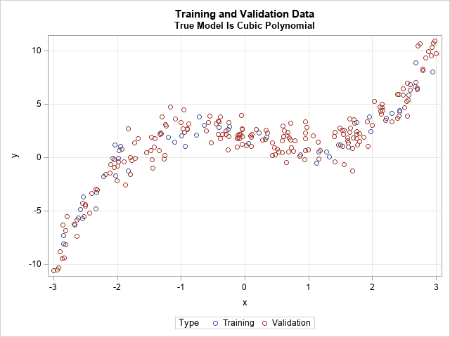
The first step of the example is to simulate data from a cubic regression model. The following SAS DATA step simulates the data. PROC SGPLOT visualizes the training and validation data.

data Have;
length Type $10.;
call streaminit(54321);
do i = 1 to 250;
   if i <= 50 then Type = "Train";       /* 50 training observations */
   else            Type = "Validate";    /* 200 validation observations */
   x = rand("uniform", -3, 3);
   /* 2 - 1.105 x - 0.2 x^2 + 0.5 x^3 */
   y = 2 + 0.5*x*(x+1.3)*(x-1.7) + rand("Normal");  /* Y = b0 + b1*X + b2*X**2 + b3*X**3 + N(0,1) */
   output;
end;
run;
 
title "Training and Validation Data";
title2 "True Model Is Cubic Polynomial";
proc sgplot data=Have;
   scatter x=x y=y / group=Type grouporder=data;
   xaxis grid;  yaxis grid;
run;

Use validation data to assess the fit

In a classical regression analysis, you would fit a series of polynomial models to the 250 observations and use a fit statistic to assess the goodness of fit. Recall that as you increase the degree of a polynomial model, you have more parameters (more degrees of freedom) to fit the data. A high-degree polynomial can produce a small sum of square errors (SSE) but probably overfits the data and is unlikely to predict future data well. To try to prevent overfitting, statistics such as the AIC and SBC include two terms: one which rewards low values of SSE and another that penalizes models that have a large number of parameters. This is done at the end of this article.

The machine learning approach is different: use some data to train the model (fit the parameters) and use different data to validate the model. A popular validation statistic is the average square error (ASE), which is formed by scoring the model on the validation data and then computing the average of the squared residuals. The GLMSELECT procedure supports the PARTITION statement, which enables you to fit the model on training data and assess the fit on validation data. The GLMSELECT procedure also supports the EFFECT statement, which enables you to form a POLYNOMIAL effect to model high-order polynomials. For example, the following statements create a third-degree polynomial model, fit the model parameters on the training data, and evaluate the ASE on the validation data:

%let Degree = 3;   
proc glmselect data=Have;
   effect poly = polynomial(x / degree=&Degree);              /* model is polynomial of specified degree */
   partition rolevar=Type(train="Train" validate="Validate"); /* specify training/validation observations */
   model y = poly / selection=NONE;                           /* fit model on training data */
   ods select FitStatistics ParameterEstimates;
run;

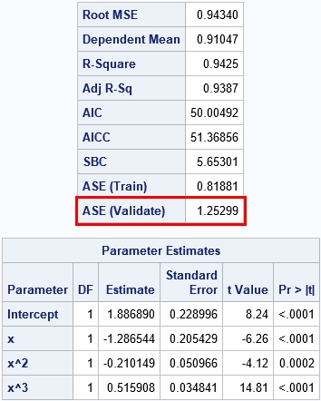
The first table includes the classical statistics for the model, evaluated only on the training data. At the bottom of the table is the "ASE (Validate)" statistic, which is the value of the ASE for the validation data. The second table shows that the parameter estimates are very close to the parameters in the simulation.

Use validation data to choose among models

You can repeat the regression analysis for various other polynomial models. It is straightforward to write a macro loop that repeats the analysis as the degree of the polynomial ranges from 1 to 7. For each model, the training and validation data are the same. If you plot the ASE value for each model (on both the training and validation data) against the degree of each polynomial, you obtain the following graph. The vertical axis is plotted on a logarithmic scale because the ASE ranges over an order of magnitude,

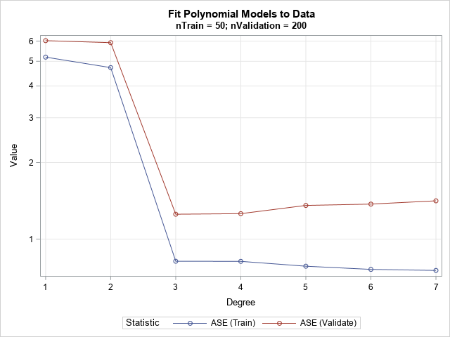
The graph shows that when you score the linear and quadratic models on the validation data, the fit is not very good, as indicated by the relatively large values of the average square error for Degree = 1 and 2. For the third-degree model, the ASE drops dramatically. Higher-degree polynomials do not substantially change the ASE. As you would expect, the ASE on the training data continues to decrease as the polynomial degree increases. However, the high-degree models, which overfit the training data, are less effective at predicting the validation data. Consequently, the ASE on the validation data actually increases when the degree is greater than 3.

Notice that the minimum value of the ASE on the validation data corresponds to the correct model. By choosing the model that minimizes the validation ASE, we have "discovered" the correct model! Of course, real life is not so simple. In real life, the data almost certainly does not follow a simple algebraic equation. Nevertheless, the graph summarizes the essence of the machine learning approach to model selection: train each model on a subset of the data and select the one that gives the smallest prediction error for the validation sample.

Classical statistics are pretty good, too!

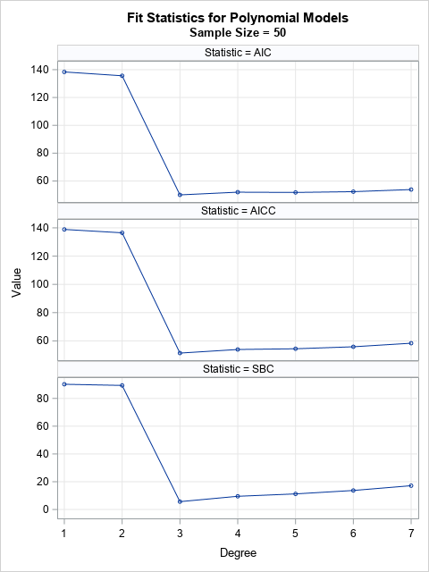
Validation methods are quite effective, but classical statistics are powerful, too. The graph to the right shows three popular fit statistics evaluated on the training data. In each case, the fit statistic reaches a minimum value for a cubic polynomial. Consequently, the classical fit statistics would also choose the cubic polynomial as being the best model for these data.

However, it's clear that the validation ASE is a simple technique that is applicable to any model that has a continuous response. Whether you use a tree model, a nonparametric model, or even an ensemble of models, the ASE on the validation data is easy to compute and easy to understand. All you need is a way to score the model on the validation sample. In contrast, it can be difficult to construct the classical statistics because you must estimate the number of parameters (degrees of freedom) in the model, which can be a challenge for nonparametric models.

Summary

In summary, a fundamental difference between classical statistics and machine learning is how each discipline assesses and compares models. Machine learning tends to fit models on a subset of the data and assess the goodness of fit by using a second subset. The average square error (ASE) on the validation data is easy to compute and to explain for models that have a continuous response. When you fit and compare several models, you can use the ASE to determine which model is best at predicting new data.

The simple example in this article also illustrates some of the fundamental principles that are used in a model selection procedure such as PROC GLMSELECT in SAS. It turns out that PROC GLMSELECT can automate many of the steps in this article. The next article shows how to use PROC GLMSELECT for model selection.

You can download the SAS program for this example.