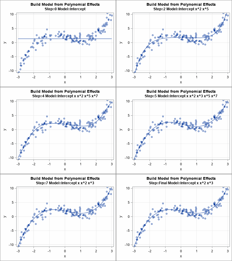
I previously discussed how you can use validation data to choose between a set of competing regression models. In that article, I manually evaluated seven models for a continuous response on the training data and manually chose the model that gave the best predictions for the validation data. Fortunately, SAS software provides ways to automate this process! This article describes how PROC GLMSELECT builds models on training data and uses validation data to choose a final model. The animated GIF to the right visualizes the sequence of models that are built.

You can download the complete SAS program that creates the results in this blog post.

How to run PROC GLMSELECT

The GLMSELECT procedure in SAS/STAT is a workhorse procedure that implements many variable-selection methods, including least angle regression (LAR), LASSO, and elastic nets. Even though PROC GLMSELECT was introduced in SAS 9.1 (Cohen, 2006), many of its options remain relatively unknown to many SAS data analysts.

Some statisticians argue against automated model building and selection. Both Cohen (2006) and the PROC GLMSELECT documentation contain a discussion of the dangers and controversies regarding automated model building. Nevertheless, machine learning techniques routinely use this sort of process to build accurate predictive models from among hundreds of variables (or features, as they are known in the ML community).

The following four statements create the analyses and graphs in this article. The (x, y) interval variables are simulated from the cubic polynomial y = 2 - 1.105*x - 0.2*x² + 0.5*x³ + N(0,1).

title "Select Model from 8 Effects";
proc glmselect data=Have seed=1 plots(StartStep=1)=(ASEPlot Coefficients);
   effect poly = polynomial(x / degree=7);    /* generate monomial effects: x, x^2, ..., x^7 */
   partition fraction(validate=0.4);          /* use 40% of data for validation */
   model y = poly / selection=stepwise(select=SBC choose=validate)
                details=steps(Candidates ParameterEstimates); /* OPTIONAL */
run;

The analysis uses the following options:

• The PLOTS= option requests two plots. The ASEPlot is a plot of the average square error (ASE) of each model on the validation data. The STARTSTEP= option displays the ASE beginning with the first step. (The zeroth step is usually the intercept-only model, which typically has a very large ASE.) The Coefficients plot shows how various effects enter or leave the model at each step of the model-building process. By default, a panel is created, but the lower part of the panel duplicates part of the ASE plot so I've unpacked the panel into separate plots.
• The EFFECT statement generates the monomial effects {x, x^2, ..., x^7} from the variable x.
• The PARTITION statement randomly divides the input data into two subsets. The validation set contains 40% of the data and the training set contains the other 60%. The SEED= option on the PROC GLMSELECT statement specifies the seed value for the random split.
• The SELECTION= option specifies the algorithm that builds a model from the effects. This example uses the stepwise selection algorithm because it is easy to understand. At each step in the model-building process, the stepwise algorithm builds a new model by modifying the model from the previous step. The new model will either contain a new effect that was not in the previous model or will remove an effect from the previous model.
• The SELECT=SBC option specifies that the procedure will use the SBC criterion to assess the candidate effects and determine which effect should be added (or removed) from the previous model.
• The CHOOSE=VALIDATE option specifies that the models are scored on the validation data. The ASE values for the models are used to choose the most predictive model from among the models that were built.
• The DETAILS= option displays information about the models that are built at each step. If you only care about the final model, you do not need this option.

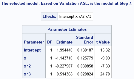
The chosen model is a cubic polynomial. The parameter estimates (below) are very close to the parameter values that are used to simulate the cubic data, so the procedure "discovered" the correct model.

How PROC GLMSELECT constructs the models

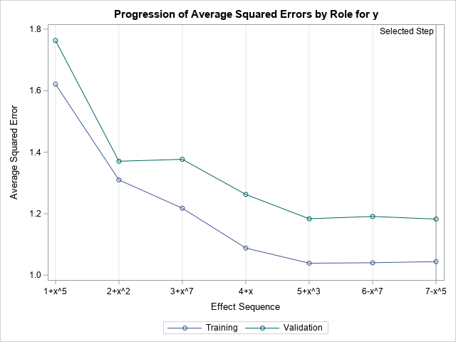
How did PROC GLMSELECT obtain that model? The output of the DETAILS=STEPS option shows that the GLMSELECT procedure built eight models. It then used the validation data to decide that the four-parameter cubic model was the model that best balances parsimony (simple versus complex models) and prediction accuracy (underfitting versus overfitting). I won't display all the output, but you can summarize the details by using the ASE plot and the Coefficients plot.

The ASE plot (shown to the right) visualizes the prediction accuracy of the models. The initial model (zeroth step) is the intercept-only model. The horizontal axis of the ASE plot shows how the models are formed from the previous model. The label for the first tick mark is "1+x^5", which means "the model at Step=1 adds the x^5 term to the previous model. The label for the second tick mark is "2+x^2", which means "the model at Step=2 adds the x^2 term to the previous model." A minus sign means that an effect is removed. For example, the label "6-x^7" means that "the model at Step=6 removes the x^7 effect from the previous model." The vertical axis tracks the change of the ASE for each successive model. The model-building process stops when it can no longer decrease the ASE on the validation data. For this example, that happens at Step=7.

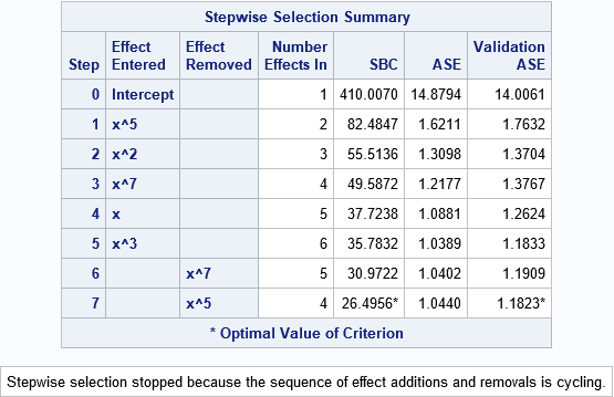
If you prefer a table, the SelectionSummary table summarizes the models that are built. The columns labeled ASE and Validation ASE contain the precise values in the ASE plot.

How PROC GLMSELECT defines the models

The models are least squares estimates for the included effects on the training data. The DETAILS=STEPS option displays the parameter estimates for each model. For these models, which are all polynomial effects for a single continuous variable, you can graph the eight models and overlay the fitted curves on the data. You can do this in eight separate plots or you can use PROC SGPLOT in SAS to create an animated gif that animates the sequence of models. The animation is shown at the top of this article.

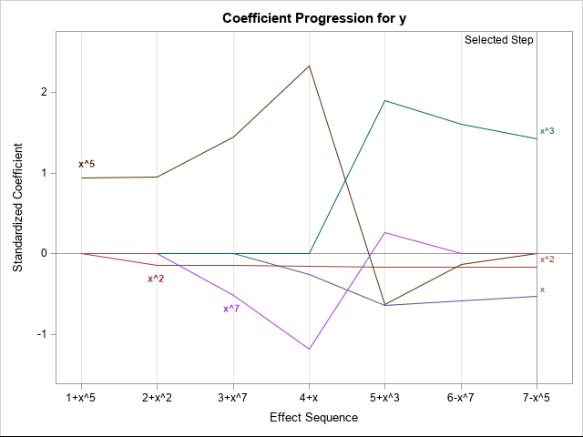
In general, you can't visualize models with many effects, but the Coefficients plot displays the values of the estimates for each model. The plot (shown to the right; click to enlarge) labels only the effects in the final model, but I have manually added labels for the x^5 and x^7 effects to help explain the plot.

Because the magnitudes of the parameter estimates can vary greatly, the vertical axis of the plot shows standardized estimates. As before, the horizontal axis represents the various models. Each line visualizes the evolution of values for a particular effect. For example, the brown line dominates the upper left portion of the graph. This line shows the progression of the standardized coefficient of the x^5 term. In models 1–4, the coefficient of the x^5 effect is large and positive. In models 5 and 6, the standardized coefficient of x^5 is small and negative. In the last model, the coefficient of x^5 is set to zero because the effect is removed. Similarly, the magenta line displays the standardized coefficients for x^7. The coefficient is negative for Steps 3 and 4, positive for Step 5, and is zero for the last two models, which do not include the x^7 effect. By using this plot, you can visually discern which effects are included in each model and study the relative change of the coefficients between models.

Summary

This article shows how to use PROC GLMSELECT in SAS to build a sequence of models for a continuous response on training data. From among the models, a final model is chosen that best predicts a validation data set. The example uses the stepwise selection technique because it is easy to understand, but the GLMSELECT procedure supports other model selection algorithms.

You can visualize the model selection process by using the ASE plot. You can visualize the progression of candidate models by using the coefficient plot. For this univariate regression model, you can also visualize each candidate model by overlaying curves or by using an animation.

For more information about the model selection procedures in SAS, see the SAS/STAT documentation or the following articles:

• Cohen, R. (2006) "Introducing the GLMSELECT PROCEDURE for Model Selection." Proceedings of the Thirty-first Annual SAS Users Group International Conference.
• Cohen, R. (2009) "Applications of the GLMSELECT Procedure for Megamodel Selection." Proceedings of the SAS Global Forum 2009 Conference.
• SAS/STAT software supports other procedures that also build models, including HPGENSELECT and (HP)QUANTSELECT. For an overview, see "Statistical model building and the SELECT procedures in SAS."