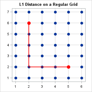
Given a rectangular grid with unit spacing, what is the expected distance between two random vertices, where distance is measured in the L₁ metric? (Here "random" means "uniformly at random.") I recently needed this answer for some small grids, such as the one to the right, which is a 7 x 6 grid. The graph shows that the L₁ distance between the points (2,6) and (5,2) is 7, the length of the shortest path that connects the two points. The L₁ metric is sometimes called the "city block" or "taxicab" metric because it measures the distance along the grid instead of "as the bird flies," which is the Euclidean distance.

The answer to the analogous question for the continuous case (a solid rectangle) is difficult to compute. The main result is that the expected distance is less than half of the diameter of the rectangle. In particular, among all rectangles of a given area, a square is the rectangle that minimizes the expected distance between random points.

Although I don't know a formula for the expected distance on a discrete regular grid, the grids in my application were fairly small so this article shows how to compute all pairwise distances and explicitly find the average (expected) value. The DISTANCE function in SAS/IML makes the computation simple because it supports the L₁ metric. It is also simple to perform computer experiments to show that among all grids that have N*M vertices, the grid that is closest to being square minimizes the expected L₁ distance.

L1 distance on a regular grid

An N x M grid contains NM vertices. Therefore the matrix of pairwise distances is NM x NM. Without loss of generality, assume that the vertices have X coordinates between 1 and N and Y coordinates between 1 and M. Then the following SAS/IML function defines the distance matrix for vertices on an N x M grid. To demonstrate the computation, the distance matrix for a 4 x 4 grid is shown, along with the average distance between the 16 vertices:

proc iml;
start DistMat(rows, cols);
   s = expandgrid(1:rows, 1:cols);   /* create (x, y) ordered pairs */
   return distance(s, "CityBlock");  /* pairwise L1 distance matrix */
finish;
 
/* test function on a 4 x 4 grid */
D = DistMat(4, 4);
AvgDist = mean(colvec(D));
print D[L="L1 Distance Matrix for 4x4 Grid"];
print AvgDist[L="Avg Distance on 4x4 Grid"];

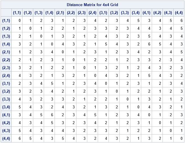
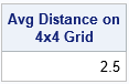
For an N x M grid, the L₁ diameter of the grid is the L₁ distance between opposite corners. That distance is always (N-1)+(M-1), which equates to 6 units for a 4 x 4 grid. As for the continuous case, the expected L₁ distance is less than half the diameter. In this case, E(L₁ distance) = 2.5.

A comparison of distances for grids of different aspect ratios

As indicated previously, the expected distance between two random vertices on a grid depends on the aspect ratio of the grid. A grid that is nearly square has a smaller expected distance than a short-and-wide grid that contains the same number of vertices. You can illustrate this fact by computing the distance matrices for grids that each contain 36 vertices. The following computation computes the distances for five grids: a 1 x 36 grid, a 2 x 18 grid, a 3 x 12 grid, a 4 x 9 grid, and a 6 x 6 grid.

/* average L1 distance on 36 x 36 grid in several configurations */
N=36;
rows = {1, 2, 3, 4, 6};
cols = N / rows;
AvgDist = j(nrow(rows), 1, .);
do i = 1 to nrow(rows);
   D = DistMat(rows[i], cols[i]);
   AvgDist[i] = mean(colvec(D));
end;
/* show average distance as a decimal and as a fraction */
numer = AvgDist*108; AvgDistFract = char(numer) + " / 108"; 
print rows cols AvgDist AvgDistFract;

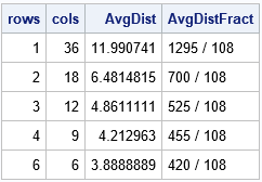
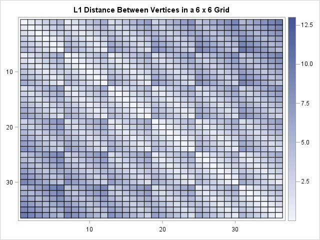
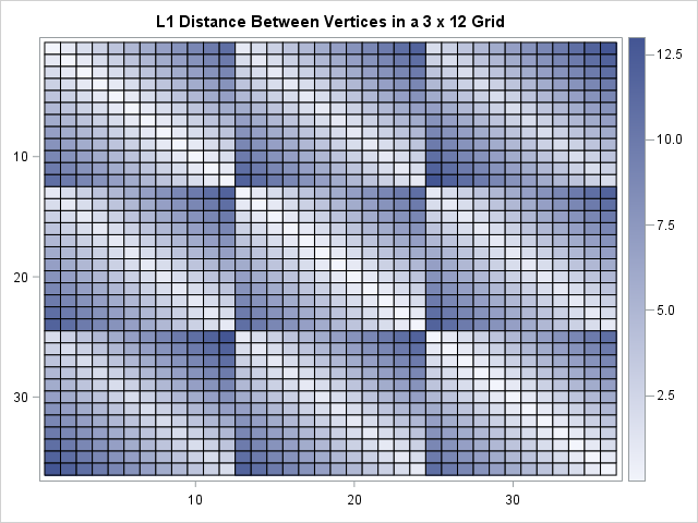
The table shows that short-and-wide tables have an average distance that is much greater than a nearly square grid that contains the same number of vertices. When the points are arranged in a 6 x 6 grid, the distance matrix naturally decomposes into a block matrix of 6 x 6 symmetric blocks, where each block corresponds to a row. When the points are arranged in a 3 x 12 grid, the distance matrix decomposes into a block matrix of 12 x 12 blocks The following heat maps visualize the patterns in the distance matrices:

D = DistMat(6, 6);
call heatmapcont(D) title="L1 Distance Between Vertices in a 6 x 6 Grid";
D = DistMat(3, 12);
call heatmapcont(D) title="L1 Distance Between Vertices in a 3 x 12 Grid";

Expected (average) distance versus number of rows

You can demonstrate how the average distance depends on the number of rows by choosing the number of vertices to be a highly composite number such as 5,040. A highly composite number has many factors. The following computation computes the average distance between points on 28 grids that each contain 5,040 vertices. A line chart then displays the average distance as a function of the number of rows in the grid:

N = 5040;               /* 5040 is a highly composite number */
rows = {1, 2, 3, 4, 5, 6, 7, 8, 9, 10, 12, 14, 15, 16, 18, 20, 
       21, 24, 28, 30, 35, 36, 40, 42, 45, 48, 56, 60, 63, 70};
cols = N / rows;
AvgDist = j(nrow(rows), 1, .);
do i = 1 to nrow(rows);
   D = DistMat(rows[i], cols[i]);
   AvgDist[i] = mean(colvec(D));
end;
 
title "Average L1 Distance Between 5040 Objects in a Regular Grid";
call series(rows, AvgDist) grid={x y} other="yaxis offsetmin=0 grid;";

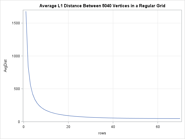
Each point on the graph represents the average distance for an N x M grid where NM = 5,040. The horizontal axis displays the value of N (rows). The graph shows that nearly square grids (rows greater than 60) have a much lower average distance than very short and wide grids (rows less than 10). The scale of the graph makes it seem like there is very little difference between the average distance in a grid with 40 versus 70 rows, but that is somewhat of an illusion. A 40 x 126 grid (aspect ratio = 3.15) has an average distance of 55.3; a 70 x 72 grid (aspect ratio = 1.03) has an average distance of 47.3.

Applications and conclusions

In summary, you can use the DISTANCE function in SAS/IML to explicitly compute the expected L₁ distance (the "city block" distance) between random points on a regular grid. You can minimize the average pairwise distance by making the grid as square as possible.

City planning provides a real-world application of the L₁ distance. If you are tasked with designing a city with N buildings along a grid, then the average distance between buildings is smallest when the grid is square. Of course, in practice, some buildings have a higher probability of being visited than others (such as a school or a grocery). You should position those buildings in the center of town to shorten the average distance that people travel.