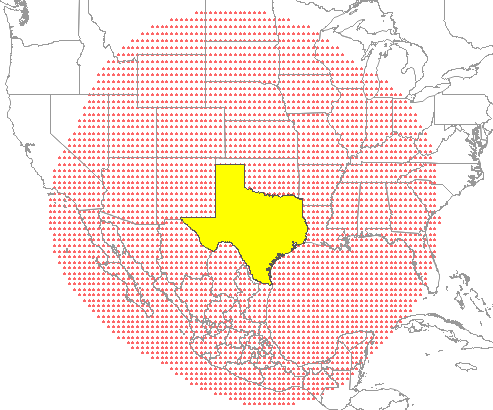
My colleague Robert Allison recently blogged about using the diameter of Texas as a unit of measurement. The largest distance across Texas is about 801 miles, so Robert wanted to find the set of all points such that the distance from the point to Texas is less than or equal to 801 miles.

Robert's implementation was complicated by the fact that he was interested in points on the round earth that are within 801 miles from Texas as measured along a geodesic. However, the idea of "thickening" or "inflating" a polygonal shape is related to a concept in computational geometry called the offset polygon or the inflated polygon. A general algorithm to inflate a polygon is complicated, but this article demonstrates the basic ideas that are involved. This article discusses offset regions for convex and nonconvex polygons in the plane. The article concludes by drawing a planar region for a Texas-shaped polygon that has been inflated by the diameter of the polygon. And, of course, I supply the SAS programs for all computations and images.

Offset regions as a union of circles and rectangles

Assume that a simple polygon is defined by listing its vertices in counterclockwise order. (Recall that a simple polygon is a closed, nonintersecting, shape that has no holes.) You can define the offset region of radius r as the union of the following shapes:

• The polygon itself
• Circles of radius r centered at each vertex
• Rectangles of width r positions outside the polygon along each edge

The following graphic shows the offset region (r = 0.5) for a convex "house-shaped" polygon. The left side of the image shows the polygon with an overlay of circles centered at each vertex and outward-pointing rectangles along each edge. The right side of the graphic shows the union of the offset regions (blue) and the original polygon (red):

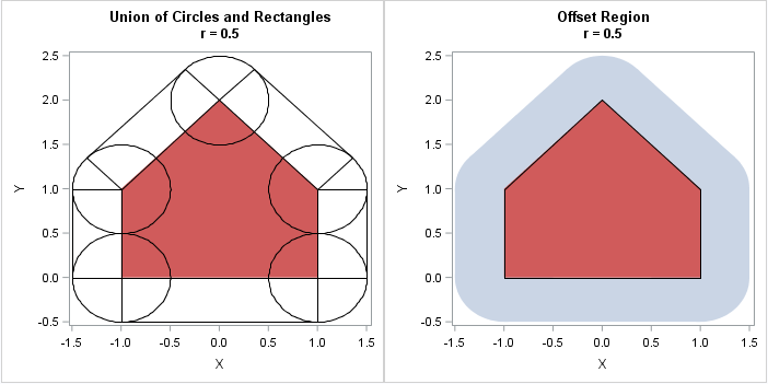
The image on the right shows why the process is sometimes called an "inflating" a polygon. For a convex polygon, the edges are pushed out by a distance r and the vertices become rounded. For large values of r, the offset region becomes a nearly circular blob, although the boundary is always the union of line segments and arcs of circles.

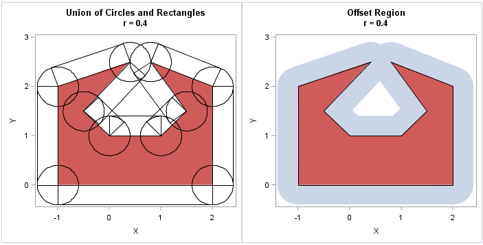
You can draw a similar image for a nonconvex polygon. The inflated region near a convex (left turning) vertex looks the same as before. However, for the nonconvex (right turning) vertices, the circles do not contribute to the offset region. Computing the offset region for a nonconvex polygon is tricky because if the distance r is greater than the minimum distance between vertices, nonlocal effects can occur. For example, the following graphic shows a nonconvex polygon that has two "prongs." Let r0 be the distance between the prongs. When you inflate the polygon by an amount r > r0/2, the offset region can contain a hole, as shown. Furthermore, the boundary of the offset regions is not a simple polygon. For larger values of r, the hole can disappear. This demonstrates why it is difficult to construct the boundary of an offset region for nonconvex polygons.

Inflating a Texas-shaped polygon

The shape of the Texas mainland is nonconvex. I used PROC GREDUCE on the MAPS.US data set in SAS to approximate the shape of Texas by a 36-sided polygon. The polygon is in a standardized coordinate system and has a diameter (maximum distance between vertices) of r = 0.2036. I then constructed the inflated region by using the same technique as shown above. The polygon and its inflated region are shown below.

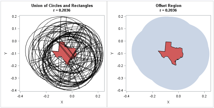
The image on the left, which shows 36 circles and 36 rectangles, is almost indecipherable. However, the image on the right is almost an exact replica of the region that appears in Robert Allison's post. Remember, though, that the distances in Robert's article are geodesic distances on a sphere whereas these distances are Euclidean distances in the plane. For the planar problem, you can classify a point as within the offset region by testing whether it is inside the polygon itself, inside any of the 36 rectangles, or within a distance r of a vertex. That computation is relatively fast because it is linear in the number of vertices in the polygon.

I don't want to dwell on the computation, but I do want to mention that it requires fewer than 20 SAS/IML statements! The key part of the computation uses vector operations to construct the outward-facing normal vector of length r to each edge of the polygon. If v is the vector that connects the i_th and (i+1)_th vertex of the polygon, then the outward-facing normal vector is given by the concise vector expression r * (v / ||v||) * M, where M is a rotation matrix that rotates by 90 degrees. You can download the SAS program that computes all the images in this article.

In conclusion, you can use a SAS program to construct the offset region for an arbitrary simple polygon. The offset region is the union of circles, rectangles, and the original polygon, which means that it is easy to test whether an arbitrary point in the plane is in the offset region. That is, you can test whether any point is within a distance r to an arbitrary polygon.