Last week I got the following message:

Dear Rick: How can I create a normal distribution within a specified range (min and max)? I need to simulate a normal distribution that fits within a specified range. I realize that a normal distribution is by definition infinite... Are there any alternatives, such as a distribution that has shape and properties similar to a normal distribution, but for which I can restrict the range? - Carol

Mathematically, this request doesn't make sense, as Carol (not her real name) acknowledges. However, if you are working with a client who is not statistically savvy, you might be asked to do the impossible! How can Carol make sense of this request?

I provide a two-part answer. First I discuss general ways to choose a distribution that models a data sample. You can use these methods when you have access to the data. Then I address the specific question and present five distributions that you can use to model data that looks like a "bounded" normal distribution. These distributions can be used when you don't have access to the data.

How to choose a distribution that matches the data?

In general, statisticians are often asked to choose a model that seems to fit an observed set of data. In simulation studies, the model is used to simulate samples that have the same distributional properties as the real data. In the book Simulating Data with SAS (Chapter 16), I discuss many strategies, including the following:

• Use domain-specific knowledge to guide you. There might be physical or biological reasons to prefer one probability distribution over another.
• Sample from the empirical distribution of the data, which is equivalent to bootstrap resampling. For more information, see the article about how to bootstrap in SAS or Chapter 15 of Simulating Data with SAS.
• Use a well-known “named” parametric distribution to model the data, such as the normal, gamma, and beta distributions. Typically you will fit several candidate distributions to the data to see which fits best. (In SAS, you can use PROC UNIVARIATE, PROC SEVERITY, or PROC NLMIXED to fit distributions.) After you choose a distribution that fits the data, you can draw random samples from the fitted distribution.
• For univariate data, you can choose a flexible system of distributions such as the Pearson system or the Johnson system. The Johnson system is supported by PROC UNIVARIATE (Wicklin, p. 112–114).
• Use a graphical tool, called the moment-ratio diagram, to help select candidate distributions for the data. Traditionally the moment-ratio diagram is a theoretical tool for understanding the relationships of families and systems of distributions, but Chapter 16 shows how to use the moment-ratio diagram as a tool to organize simulation studies.

These ideas (and others) are illustrated in the following diagram, which is also from Wicklin (2013, p. 298):

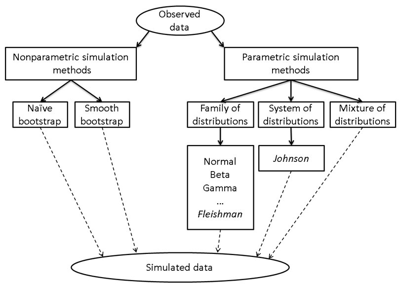
The flowchart shows a few paths that a researcher can follow to model data. Most of the paths are also applicable to multivariate data.

Simulate data from the "eyeball distribution"

Now let's discuss the specific question that I was asked: how to simulate a "bounded" normal distribution. If Carol has access to the data, she could use the techniques in the previous section. Consequently, I assume that Carol does not have access to the data. This can happen in several ways, such as when you are trying to reproduce the results in a published article but the article includes only summary statistics or a graph of the data. If you cannot obtain the original data from the authors, you might be forced to simulate fake data based only on the graph and the summary statistics.

I call this using the "eyeball distribution." For non-native speakers of English, "to eyeball" means to look at or observe something. When used as an adjective, “eyeball” indicates that a quantity was obtained by visual inspection, rather than through formal measurements. Thus an "eyeball distribution" is one that is chosen heuristically because it looks similar to the histogram of the data. (You can extend these ideas to multivariate data.)

From Carol's description, the histogram of her data is symmetric, unimodal, and "bell-shaped." The data are in the interval [a, b]. I can think of several "eyeball distributions" that could model data like this:

1. If you know the sample mean (m) and standard deviation (s), then draw random samples from N(m, s).
2. If you know sample quantiles of the data, you can approximate the CDF and use inverse probability sampling for the simulation.
3. Theory tells us that 99.7% of the normal distribution is within three standard deviations of the mean. For symmetric distributions, the mean equals the midrange m = (a + b)/2. Thus you could use the three-sigma rule to approximate s ≈ (b - a)/6 and sample from N(m, s).
4. If you have domain knowledge that guarantees that the data are truly bounded on [a, b], you could use the truncated normal distribution, which samples from N(m, s) but discards any random variates that are outside of the interval.
5. Alternatively, you can sample from a symmetric bounded distribution such as the Beta(α, α) distribution. For example, Beta(5, 5) is approximately bell-shaped on the interval [0,1].

The first option is often the most reasonable choice. Even though the original data are in the interval [a, b], the simulated data do not have to be in the same interval. If you believe that the original data are normally distributed, then simulate from that model and accept that you might obtain simulated data that are beyond the bounds of the original sample. The same fact holds for the third option, which estimates the standard deviation from a histogram.

The following SAS DATA step implements the last three options. The sample distributions are displayed by using a comparative histogram in SAS:

%let N = 500;      /* sample size */
%let min = 5;
%let max = 15;
 
proc format;
value MethodFmt 1 = "Normal, 3-Sigma Rule"
                2 = "Truncated Normal"
                3 = "Beta(5, 5), Scaled";
run;
data BellSim(keep=x Method);
format method MethodFmt.;
call streaminit(54321);  /* set random number seed */
numSD = 3;               /* use 3-sigma rule to estiamte std dev */
mu = (&min + &max)/2;
sigma = (&max - &min)/ (2*numSD);
 
method = 1;        /* Normal distribution N(mu, sigma) */
   do i = 1 to &N;
      x = rand("Normal", mu, sigma);  output;
   end;
 
method = 2;        /* truncated normal distribution TN(mu, sigma; a, b) */
   i = 0;
   do until (i = &N);
      x = rand("Normal", mu, sigma);
      if &min < x < &max then do;
         output;
         i + 1;
      end;
   end;
 
method = 3;        /* symmetric beta distribution, scaled into [a, b] */
   alpha = 5;
   do i = 1 to &N;
      x = &min + (&max - &min)*rand("beta", alpha, alpha);
      output;
   end;
run;
 
ods graphics / width=480px height=480px;
title "Simulate Bell-Shaped Data on [&min, &max]";
proc sgpanel data=BellSim;
   panelby method / columns=1 novarname;
   histogram x;
   refline &min &max / axis=x;
   colaxis values=(&min to &max) valueshint;
run;

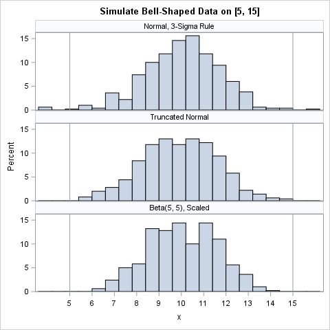
The histograms show a simulated sample of size 500 for each of the three models. The top sample is from the normal distribution. It contains simulated observations that are outside of the interval [a,b]. In many situations, that is fine. The second sample is from the truncated normal distribution on [a,b]. The third is from a Beta(5,5) distribution, which has been scaled onto the interval [a,b].

Although the preceding SAS program answers the question Carol asked, let me emphasize that if you (and Carol) have access to the data, you should use it to choose a model. When the data are unobtainable, you can use an "eyeball distribution," which is basically a guess. However, if your goal is to generate fake data so that you can test a computational method, an eyeball distribution might be sufficient.