When modeling and simulating data, it is important to be able to articulate the real-life statistical process that generates the data.

Suppose a friend says to you, "I want to simulate two random correlated variables, X and Y." Usually this means that he wants data generated from a multivariate distribution, such as the bivariate normal distribution. However, an alternative scenario is to generate X by according to some univariate distribution and generate Y according to some regression model.

In both cases, the variables are related. However, in the first case the pairs are generated from a joint bivariate distribution. In the second case, Y is assumed to be a response variable that depends on X. In this case, you are generating Y conditionally based on the value of X. Usually asking your friend about the sampling framework of the real data enables you to determine which model and simulation is more appropriate.

Similarly, you can make various assumptions about the data in a contingency table (sometimes called a frequency table or a cross-tabulation), which lead to different models. The fundamental question is "how were the data generated or collected?" The answer to that question should become the basis for modeling and simulating the data.

The following are some common assumptions about the sampling framework for data in contingency tables (Stokes, Davis, and Koch, 2012, Chapter 2):

1. Assume that the sample size is fixed, but the rows and column sums are not. For example, the Wikipedia article on contingency tables includes a table that shows the gender and handedness (right handed or left handed) of 100 random people. If you choose a new sample of 100 people, it is unlikely that the row or column sums will be the same. You can use the multinomial distribution to simulate these tables.


2. Assume that the rows sums are fixed but the column sums are not. A modification of the previous survey design is to interview 50 men and 50 women and ask each person whether they are right or left handed. This design fixes the number of men and women, and any simulation of this data must respect the design. You can use the binomial distribution to simulate these tables row by row.


3. Assume that the row and column sums are fixed. This assumption is often used when you want to evaluate a statistical hypothesis on the data. For example, Fisher's exact test computes an exact p-value by considering all tables that have the same row and column sums as the observed table, and then counts the proportion of tables whose test statistic is equal to or more extreme than the observed value. You can use the hypergeometric distribution to simulate random tables 2 x 2 tables with specified marginal distributions.

These techniques generalize to larger tables. For the first assumption (fixed sample size) you can use the multinomial distribution to generate each cell count. For the second assumption (fixed row sums), there are a multitude of ways to model a response variable, including log-linear models. For details, see Friendly (2000, Chapter 7) or Stokes, Davis, and Koch (2012).

The third assumption (fixed row and column marginal sums) is tractable for a 2 x 2 table, but generating all tables becomes infeasible for large tables. However, if you can simulate random tables that have a specified marginal sums, then you can obtain a Monte Carlo estimate for the p-value of the test. Let's see how to simulate such tables.

The PROC FREQ documentation contains a 2 x 2 table for 23 patients in a case-control study relating dietary fat and heart disease. The column sums are {13 10} and the row sums are {15 8}. The following statements simulate three tables that have the same row and column sums:

proc iml;
/* first arg is row vector of sums of cols; second arg contains sums of rows */
start RandContingency2x2(_c, _r);
   c = rowvec(_c);
   r = colvec(_r);
   if ncol(c)^=2 | nrow(r)^=2 then 
      abort "This function applies only to 2x2 tables";
   tbl = j(2, 2, 0);           /* allocate 2x2 table */
   call randgen(a, "Hyper", sum(r), r[1], c[1]);  
   tbl[1,1] = a;               /* assign random value to first element */
   tbl[2,1] = c[1] - a;        /* constraint on column sum */
   tbl[ ,2] = r - tbl[ ,1];    /* constraints on row sums */
   return( tbl );
finish;
 
call randseed(1);
/* marginals from PROC FREQ example */
c = {13 10};                  /* sum of columns */
r = {15, 8};                  /* sum of rows */
do i = 1 to 3;
   tbl = RandContingency2x2(c, r);
   print tbl;
end;

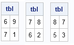
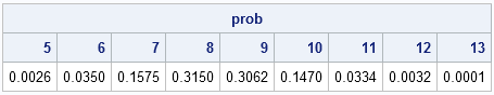
The output shows three of the nine unique tables that satisfy the specified marginal sums. You can use the PDF function for the hypergeometric distribution to show that the first table is generated with probability 0.035, the second table has the probability 0.1575, and the third appears with probability 0.315. The following statement computes the probabilities for all 2 x 2 tables where the upper left cell has the specified values:

/* prob of 2x2 table with row sums (r) and col sums (c) where A[1,1]=5,6,...13 */
prob = pdf("Hyper", 5:13, sum(r), r[1], c[1]);
print prob[c=("5":"13") F=6.4];

In a future blog post, I will discuss how to generalize this simulation to larger tables that have r rows and c columns.