How do you simulate a contingency table that has a specified row and column sum? Last week I showed how to simulate a random 2 x 2 contingency table when the marginal frequencies are specified. This article generalizes to random r x c frequency tables (also called cross-tabulations) that have the same marginal row and column sums as an observed table of counts.

For example, consider the following table:

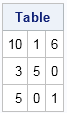
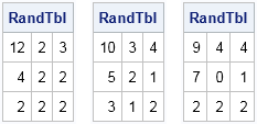
The column sums are c = {18 6 7} and the row sums are r = {17, 8, 6}. There are many other tables that have the same row sums and column sums. For example, the following three tables satisfy those conditions:

In a previous blog post, I presented a standard algorithm (see Gentle, 2003, p. 206) that can generate an r x c table one column at a time. The first column is a random draw from the multivariate hypergeometric distribution with a total number of elements equal to the observed count for that column. After generating the first column, you subtract the counts from the marginal row counts. You then iteratively apply the same algorithm to the second column, and so forth.

The hypergeometric algorithm requires some special handling for certain degenerate situations. In contrast, a simpler algorithm from the algorithm of Agresti, Wackerly, and Boyett (1979) is mathematically equivalent but easier to implement. You can download a SAS/IML program that implements both these algorithms.

Assume the columns sums are given by the vector c = {c₁, c₂, ..., c_m} and the row sums are given by r = {r₁, r₂, ..., r_n}. Think about putting balls of m different colors into an urn. You put in c₁ balls of the first color, c₂ balls of the second color, and so forth. Mix up the balls. Now pull out r₁ balls, count how many are of each color, and write those numbers in the first row of a table. Then pull out r₂ balls, record the color counts in the second row of the table, and so forth.

The following SAS/IML module implements the algorithm in about 15 lines of code. For your convenience, the code includes the definition of TabulateLevels function, which counts the balls of every color, even if some colors have zero counts:

proc iml;
/* Output levels and frequencies for categories in x, including all reference levels. 
   https://blogs.sas.com/content/iml/2015/10/07/tabulate-counts-ref.html */
start TabulateLevels(OutLevels, OutFreq, x, refSet);
   call tabulate(levels, freq, x);        /* compute the observed frequencies */
   OutLevels = union(refSet, levels);     /* union of data and reference set */ 
   idx = loc(element(OutLevels, levels)); /* find the observed categories */
   OutFreq = j(1, ncol(OutLevels), 0);    /* set all frequencies to 0 */
   OutFreq[idx] = freq;                   /* overwrite observed frequencies */
finish;
 
/* Algorithm from Agresti, Wackerly, and Boyett (1979), Psychometrika */
start RandContingency(_c, _r);
   c = rowvec(_c);   m = ncol(c);
   r = colvec(_r);   n = nrow(r);
   tbl = j(n, m, 0);
   refSet = 1:m;
   vals = repeat(refSet, c);    /* vector replication: https://blogs.sas.com/content/iml/2014/07/07/expand-frequency-data.html */
   perm = sample(vals, ,"WOR"); /* n=number of elements of vals */
   e = cusum(r);                /* ending indices */
   s = 1 // (1+e[1:n-1]);       /* starting indices */
   do j = 1 to n;
      v = perm[ s[j]:e[j] ];    /* pull out r1, r2, etc */
      call TabulateLevels(lev, freq, v, refSet);
      tbl[j, ] = freq;          /* put counts in jth row */
   end;
   return( tbl );
finish;

Every time you call the RandContingency function it generates a random table with the specified row and column sums. The following statements define a 3 x 3 table and generate three random tables, which appear at the beginning of this article. Each random table is a draw from the null distribution that assumes independence of rows and columns:

call randseed(12345);
Table = {10 1 6,
          3 5 0,
          5 0 1};
c = Table[+, ];
r = Table[ ,+];
do i = 1 to 3;
   RandTbl = RandContingency(c, r);
   print RandTbl;
end;

The example is small, but the algorithm can handle larger tables, both in terms of the dimension of the table and in terms of the sample size. For example, the following example defines row and column sums for a 500 x 20 table. The sample size for this table is 30,000.

/* try a big 500 x 20 table */
r = j(500,  1,   60);
c = j(  1, 20, 1500);
tbl = RandContingency(c, r);
ods graphics / width=600px height=2000px;
call heatmapcont(tbl);

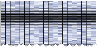
The table is too big to print in this article, but you can create a heat map to that shows the distribution of values. The adjacent image shows the first 40 rows of the heat map. The cells in the table vary between 0 (white) and 11 (dark blue), with about half of the cells having values 3 or 4. For tables of this size, you can create thousands of tables in a few seconds. For smaller tables, you can simulate ten thousands tables in less than a second.

In a future blog post I will show how to use the RandContingency function to simulate random tables and carry out Monte Carlo estimation of exact p-values.