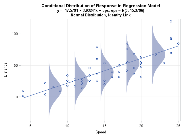
A friend who teaches courses about statistical regression asked me how to create a graph in SAS that illustrates an important concept: the conditional distribution of the response variable. The basic idea is to draw a scatter plot with a regression line, then overlay several probability distributions along the line, thereby illustrating the model assumptions about the distribution of the response for each value of the explanatory variable.

For example, the image at left illustrates the theoretical assumptions for ordinary linear regression (OLS) with homoscedastic errors. The central line represents the conditional mean of the response. The observed responses are assumed to be of the form y_i = β₀ + β₁x_I + ε_i where ε_i ∼ N(0, σ) for some value of σ. The normal distributions all have the same variance and are centered on the regression line. Pictures like this are used by instructors and textbook authors to illustrate the assumptions of linear regression. You can create similar pictures for variations such as heteroscedastic errors or generalized linear models.

This article outlines how to create the graph in SAS by using the SGPLOT procedure. The data are from a blog post by Arthur Charpentier, "GLM, non-linearity and heteroscedasticity," as are some of the ideas. Charpentier also inspired a related post by Markus Gesmann, "Visualising theoretical distributions of GLMs." Thanks to Randy Tobias and Stephen Mistler for commenting on an early draft of this post.

Fitting and scoring a regression model

Charpentier uses a small data set that contains the stopping distance (in feet) when driving a car at a certain speed (in mph). The OLS regression model assumes that distance (the response) is a linear function of speed and that the observed distances follow the previous formula.

In order to make the program as clear as possible, I have used "X" as the name of the explanatory variable and "Y" as the name of the response variable. I have used macro variables in a few places in order to clarify the logic of the program. However, to prevent the program from appearing too complicated, I did not fully automate the process of generating the graph.

The following statements define the data and use PROC SQL to create macro variables that contain the minimum and maximum value of the explanatory variable. Then a DATA step creates 101 equally spaced points in the interval [min(x), max(x)], which will be used to score the regression model:

/* data and ideas from http://freakonometrics.hypotheses.org/9593 */
/* Stopping distance (ft) for a car traveling at certain speeds (mph) */
data MyData(label="cars data from R");
input x y @@;
logY = log(y);
label x = "Speed (mph)"  y = "Distance (feet)" logY = "log(Distance)";
datalines;
4   2  4 10  7  4  7  22  8 16  9 10 10 18 10 26 10  34 11 17 
11 28 12 14 12 20 12  24 12 28 13 26 13 34 13 34 13  46 14 26 
14 36 14 60 14 80 15  20 15 26 15 54 16 32 16 40 17  32 17 40 
17 50 18 42 18 56 18  76 18 84 19 36 19 46 19 68 20  32 20 48 
20 52 20 56 20 64 22  66 23 54 24 70 24 92 24 93 24 120 25 85 
;
 
/* 1. Create scoring data set */
/* 1a. Put min and max into macro variables */
proc sql noprint;
  select min(x), max(x) into :min_x, :max_x 
  from MyData;
quit;
 
/* 1b. Create scoring data set */
data ScoreX;
do x = &min_x to &max_x by (&max_x-&min_x)/100;  /* min(X) to max(X) */
   output;
end;
run;

The next statements call PROC GENMOD to fit an OLS model. (I could have used PROC GLM or REG for this model, but in a future blog post I want to explore generalized linear models.) The procedure outputs the parameter estimates, as shown, and use the STORE statement to save the OLS model to a SAS item store. The PLM procedure is used to score the model at the points in the ScoreX data set. (For more about PROC PLM, see Tobias and Cai (2010).) The fitted values are saved to the SAS data set Model:

/************************************************/
/* Model 1: linear regression of Y              */
/************************************************/
title "Linear Regression of Y";
/* Create regression model. Save model to item store. Score with PROC PLM. */
proc genmod data=MyData;
  model y = x / dist=normal link=identity;
  ods select ParameterEstimates;
  store work.YModel / label='Normal distribution for Y; identity link';
run;
 
proc plm restore=YModel noprint;
  score data=ScoreX out=Model pred=Fit; /* score model; save fitted values */
run;

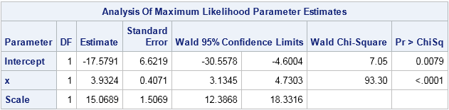
The estimate for the intercept is b₀ = -17.58 and the estimate for the linear coefficient is b₁ = 3.93. The Scale value is an MLE estimate for the standard deviation of the error distribution. These estimates will be used to plot a sequence of normal distributions along a fitted response curve that is overlaid on the scatter plot. If you use PROC GLM to fit the model, the RMSE statistic is a (slightly different) estimate for the scale parameter.

Plotting conditional distributions

The next step is to create data for a sequence of normal probability distributions that are spaced along the X axis and have standard deviation σ=15.07. Charpentier plots the distributions in three dimensions, but many authors simply let each distribution "fall on its side" and map the density scale into the coordinates of the data. This requires scaling the density to transform it into the data coordinate system. In the following DATA step, the maximum height of the density is half the distance between the distributions. The distributions are centered on the regression line, and extend three standard deviations in either direction. The PDF function is used to compute the density distribution, centered at the conditional mean, for the response variable.

The following code supports a link function, such as a log link. For this analysis, which uses the identity link, the ILINK macro variable is set to blank. However, for a generalized linear model with a log link, you can set the inverse link function to EXP.

/* specify parameters for model */
%let std = 15.3796;
%let b0 = -17.5791;
%let b1 =   3.9324;
%let ILINK = ;            /* blank for identity link; for log link use EXP */
 
/* create values to plot the assumed response distribution */
data NormalResponse(keep = s t distrib);
/* compute scale factor for height of density distributions */
ds = (&max_x - &min_x) / 6;          /* spacing for 5 distributions */
maxHt = ds / 2;                      /* max ht is 1/2 width */
maxPdf = pdf("Normal", 0, 0, &std);  /* max density for normal distrib */
ScaleFactor = maxHt / maxPDF;        /* scale density into data coords */
/* place distribs horizontally along X scale */
do s = (&min_x+ds) to (&max_x-ds) by ds;
   eta = &b0 + &b1*s;                /* linear predictor */
   pred = &ILINK(eta);               /* apply inverse link function */
   /* compute distribution of Y | X. Assume +/-3 std dev is appropriate */
   do t = pred - 3*&std to pred + 3*&std by 6*&std/50; 
      distrib = s + ScaleFactor * pdf("Normal", t, pred, &std); 
      output;
   end;
end;
run;

The last step is to combine the original data, the regression line, and the probability distributions into a single data set. You can then use PROC SGPLOT to create the graph shown at the top of the article. The data are plotted by using the SCATTER statement, the regression line is overlaid by using the SERIES statement, and the BAND statement is used to plot the sequence of semi-transparent probability distributions along the regression line:

/* merge data, fit, and error distribution information */
data All;  set MyData Model NormalResponse;  run;
 
title "Conditional Distribution of Response in Regression Model";
title2 "y = &b0 + &b1*x + eps, eps ~ N(0, &std)";
title3 "Normal Distribution, Identity Link";
proc sgplot data=All noautolegend;
  scatter x=x y=y;
  series x=x y=Fit;
  band y=t lower=s upper=distrib / group=s
       transparency=0.4 fillattrs=GraphData1;
  xaxis grid;
  yaxis grid;
run;
title;

The program could be shorter if I use the SAS/IML language, but I wanted to make the program available to as many SAS users as possible, so I used only Base SAS and procedures in SAS/STAT. The graph at the beginning of this article illustrates the basic assumptions of ordinary linear regression. Namely, for a given value of X, the OLS model assumes that each observed Y value is an independent random draw from a normal distribution centered at the predicted mean. The homoscedastic assumption is that the width of those probability distributions is constant.

In a future blog post I will draw a similar picture for a generalized linear model that has a log link function.