In a previous post, I used statistical data analysis to estimate the probability that my grocery bill is a whole-dollar amount such as $86.00 or $103.00. I used three weeks' grocery receipts to show that the last two digits of prices on items that I buy are not uniformly distributed. (The prices tend to be values such as $1.49 or $1.99 that appear to be lower in price.) I also showed that sales tax increases the chance of getting a whole-dollar receipt.
In this post, I show how you can use resampling techniques in SAS/IML software to simulate thousands of receipts. You can then estimate the probability that a receipt is a whole-dollar amount, and use bootstrap ideas to examine variation in the estimate.
Simulating Thousands of Receipts
The SAS/IML language is ideal for sampling and simulation in the SAS environment. I previously introduced a SAS/IML module called SampleReplaceUni which performs sampling with replacement from a set. You can use this module to resample from the data.
First run a SAS DATA step program to create the WORK.PRICES data set. The ITEM variable contains prices of individual items that I buy. You can resample from these data. I usually buy about 40 items each week, so I'll use this number to simulate a receipt.
The following SAS/IML statements simulate 5,000 receipts. Each row of the y vector contains 40 randomly selected items (one simulated receipt), and there are 5,000 rows. The sum across the rows are the pre-tax totals for each receipt:
proc iml;
/** read prices of individual items **/
use prices; read all var {"Item"}; close prices;

SalesTax = 0.0775;   /** sales tax in Wake county, NC **/
numItems = 40;       /** number of items in each receipt **/
NumResamples = 5000; /** number of receipts to simulate **/
call randseed(4321);

/** LOAD or define the SampleReplaceUni module here. **/

/** resample from the original data. **/
y = sampleReplaceUni(Item`, NumResamples, NumItems);
pretax = y[,+];       /** sum is get pre-tax cost of each receipt **/
total = round((1 + SalesTax) # pretax, 0.01); /** add sales tax **/
whole = (total=int(total)); /** indicator: whole-dollar receipts **/
Prop = whole[:];    /** proportion that are whole-dollar amounts **/
print NumItems NumResamples (sum(whole))[label="Num00"]
Prop[format=PERCENT7.2 label="Pct"]; |
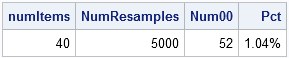
The simulation generated 52 whole-dollar receipts out of 5,000, or about 1%.
Estimating the Probability of a Whole-Dollar Receipt
The previous computation is the result of a single simulation. In technical terms, it is a point-estimate for the probability of obtaining a whole-dollar receipt. If you run another simulation, you will get a slightly different estimate. If you run, say, 200 simulations and plot all of the estimates, you obtain the sampling distribution for the estimate. For example, you might obtain something that looks like the following histogram:
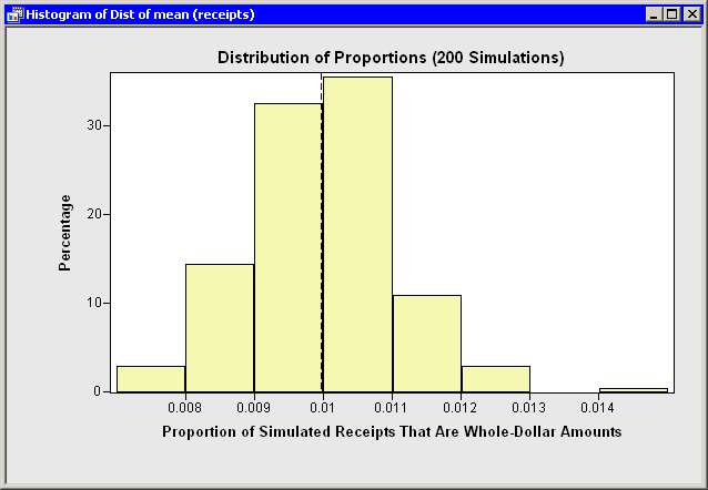
The histogram shows the estimates for 200 simulations. The vertical dashed line in the histogram is the mean of the 200 estimates, which is about 1%. So, on average, I should expect my grocery bills to be a whole-dollar amount about 1% of the time. The histogram also indicates how the estimate varies over the 200 simulations.
The Bootstrap Distribution of Proportions
The technique that I've described is known as a resampling or bootstrap technique.
In the SAS/IML language, it is easy to wrap a loop around the previous simulation and to accumulate the result of each simulation. The mean of the accumulated results is a bootstrap estimate for the probability that my grocery receipt is a whole-dollar amount. You can use quantiles of the accumulated results to form a bootstrap confidence interval for the probability. For example:
NumRep = 200;          /** number of bootstrap replications **/
Prop = j(NumRep, 1);   /** allocate vector for results **/
do k = 1 to NumRep;
   /** resample from the original data **/
   ...
   /** proportion of bills that are whole-dollar amounts **/
   Prop[k] = whole[:];
end;

meanProp = Prop[:];
/** LOAD or define the Qntl module here **/
call Qntl(q, Prop, {0.05 0.95});
print numItems meanProp q[label="90% CI"]; |
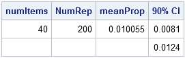
Notice that 90% of the simulations had proportions that are between 0.81% and 1.24%. I can use this as a 90% confidence interval for the true probability that my grocery receipt will be a whole-dollar amount.
You can download the complete SAS/IML Studio program that computes the estimates and creates the histogram.
Conclusions
My intuition was right: I showed that the chance of my grocery receipt being a whole-dollar amount is about one in a hundred. But, more importantly, I also showed that you can use SAS/IML software to resample from data, run simulations, and implement bootstrap methods.
What's next? Well, all this programming has made me hungry. I’m going to the grocery store!

2 Comments
This is way cool analysis. I wait all week to read the end. I'm examining next 100 shopping bills and see if I get one.
wow,this is pretty cool.this obviously took a lot of effort.well done.