Normal, Poisson, exponential—these and other "named" distributions are used daily by statisticians for modeling and analysis. There are four operations that are used often when you work with statistical distributions. In SAS software, the operations are available by using the following four functions, which are essential for every statistical programmer to know:

• PDF function: This function is the probability density function. It returns the probability density at a given point for a variety of distributions. (For discrete distribution, the PDF function evaluates the probability mass function.)
• CDF function: This function is the cumulative distribution function. The CDF returns the probability that an observation from the specified distribution is less than or equal to a particular value. For continuous distributions, this is the area under the PDF up to a certain point.
• QUANTILE function: This function is closely related to the CDF function, but solves an inverse problem. Given a probability, P, it returns the smallest value, q, for which CDF(q) is greater than or equal to P.
• RAND function: This function generates a random sample from a distribution. In SAS/IML software, use the RANDGEN subroutine, which fills up an entire matrix at once.

The probability density function (PDF)

The probability density function is the function that most people use to define a distribution. For example, the PDF for the standard normal distribution is φ(x) = (1/ √2π ) exp(-x²/2). You can use the PDF function to draw the graph of the probability density function. For example, the following SAS program uses the DATA step to generate points on the graph of the standard normal density, as follows:

data pdf;
do x = -3 to 3 by 0.1;
   y = pdf("Normal", x);
   output;
end;
x0 = 0; pdf0 = pdf("Normal", x0); output;
x0 = 1; pdf0 = pdf("Normal", x0); output;
run;
 
proc sgplot data=pdf noautolegend;
title "Normal Probability Density";
series x=x y=y;
scatter x=x0 y=pdf0;
vector x=x0 y=pdf0 /xorigin=x0 yorigin=0 noarrowheads lineattrs=(color=gray);
xaxis grid label="x"; yaxis grid label="Normal PDF";
refline 0 / axis=y;
run;

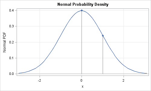
The plot shows the graph of the PDF, and shows that PDF(0) is a little less than 0.4 and PDF(1) is close to 0.25.

The cumulative distribution function (CDF)

The mathematical basis for statistics is probability. The cumulative distribution function returns the probability that a value drawn from a given distribution is less than or equal to a given value.

For a continuous distribution, the CDF is the integral of the PDF from the lower range of the distribution (often -∞) to the given value. For example, the CDF of zero for the standard normal is 0.5, because the area under the normal curve to the left of zero is 0.5. For a discrete distribution, the CDF is the sum of the PDF (mass function) for all values less than or equal to the given value.

The CDF of any distribution is a non-decreasing function. For the familiar continuous distributions, the CDF is monotone increasing. For discrete distributions, the CDF is a step function. The following DATA step generates points on the graph of the standard normal CDF:

data cdf;
do x = -3 to 3 by 0.1;
   y = cdf("Normal", x);
   output;
end;
x0 = 0;     cdf0 = cdf("Normal", x0); output;
x0 = 1.645; cdf0 = cdf("Normal", x0); output;
run;
 
ods graphics / height=500;
proc sgplot data=cdf noautolegend;
title "Normal Cumulative Probability";
series x=x y=y;
scatter x=x0 y=cdf0;
vector x=x0 y=cdf0 /xorigin=x0 yorigin=0 noarrowheads lineattrs=(color=gray);
vector x=x0 y=cdf0 /xorigin=-3 yorigin=cdf0 noarrowheads lineattrs=(color=gray);
xaxis grid label="x";
yaxis grid label="Normal CDF" values=(0 to 1 by 0.05);
refline 0 1/ axis=y;
run;

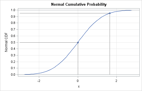
The graph shows that CDF(0) is 0.5 and CDF(1.645) is 0.95.

The quantile (inverse CDF) function

If the CDF is continuous and strictly increasing, there is a unique answer to the question: Given an area (probability), what is the value, q for which the integral up to q has the specified area? The value q is called the quantile for the specified probability distribution. The median is the quantile of 0.5, the 90th percentile is the quantile of 0.9, and so forth. For discrete distributions, the quantile is the smallest value for which the CDF is greater than or equal to the given probability.

For the standard normal distribution, the quantile of 0.5 is 0, and the 95th percentile is 1.645. You can find a quantile graphically by using the CDF plot: choose a value q between 0 and 1 on the vertical axis, then use the CDF curve to find the value of x whose CDF is q.

Quantiles are used to compute p-values for hypothesis testing. For symmetric distributions, such as the normal distribution, the quantile for 1-α/2 is used to compute two-sided p-values. For example, when α=0.05, the (1-α/2) quantile for the standard normal distribution is quantile("Normal", 0.975), which is the famous number 1.96.

Random samples with the RAND function

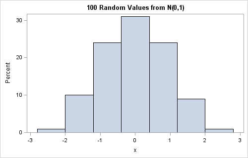
The RAND function (and the RANDGEN subroutine in the SAS/IML language) enables you to generate a random sample from a given distribution. I have written about random samples many times, including a recent post on random number streams in SAS. The following DATA step calls the STREAMINIT subroutine to set a random number stream and samples 100 random values from the standard normal distribution. (If you use SAS/IML, the analogous subroutines are RANDSEED and RANDGEN.) A histogram of the results follows:

data rand;
call streaminit(12345);
do i = 1 to 100;
   x = rand("Normal");
   output;
end;
run;
 
proc sgplot data=rand;
title "100 Random Values from N(0,1)";
histogram x;
run;

Comparison with other languages

No matter what statistical language you use, these four operations are essential. In the R language, these functions are known as the dxxx, pxxx, qxxx, and rxxx functions, where xxx is the suffix used to specify a distribution. For example, the four R functions for the normal distribution are named dnorm, pnorm, qnorm, and rnorm. In the MATLAB language, these four functions are named pdf, cdf, icdf, and random.

Long-time SAS users might remember the older PROBXXX, XXXINV, and RANXXX functions for computing the CDF, inverse CDF (quantiles), and for sampling. For example, you can use the PROBGAM, GAMINV, and RANGAM functions for working with the gamma distribution. (For the normal distribution, the older names are PROBNORM, PROBIT, and RANNOR.) Because the older RANXXX functions use an older random number generator, I do not recommend them for generating many millions of random values.