If not for probability theory, urns would appear only in funeral homes and anthologies of British poetry.

But in probability and statistics, urns are ever present and contain colored balls. The removal and inspection of colored balls from an urn is a classic way to demonstrate probability, sampling, variation, and other elementary concepts in probability and statistics.

This article describes some ball-and-urn experiments, and how you can use SAS software to simulate drawing balls from an urn under various assumptions. This article describes the case where the urn contains exactly two colors, often chosen to be black and white. A subsequent article will describe the case where the urn contains more than two colors.

Let K₀ be the number of black balls, K₁ be the number of white balls, and N be the total number of balls in the urn.

Bernoulli Trials

The simplest experiment is to reach into the urn and pull out a single ball. Although there are two kinds of balls, the act of drawing one ball depends only on one parameter, namely the probability of choosing a white ball, which is p = K₁ / N. (Similarly, the ball will be black with probability 1–p.) This is called a Bernoulli trial. In SAS the Bernoulli distribution is supported by the four essential functions for probability and sampling: the PDF, CDF, QUANTILE, and RAND functions.

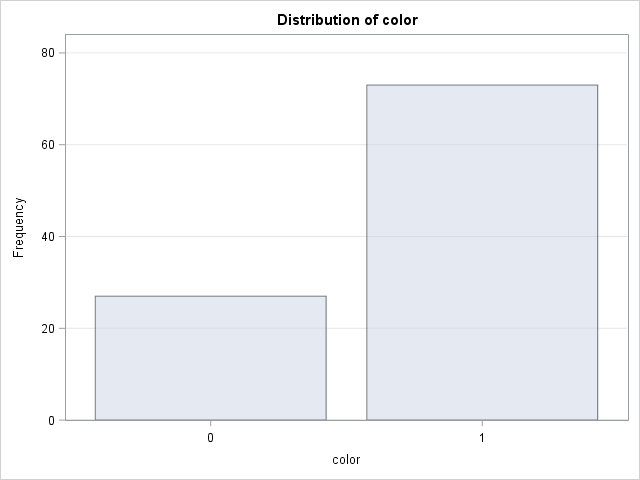
For example, the following DATA step repeats 100 independent Bernoulli trials and plots the results for an urn in which 75% of the balls are white. "Independence" means that after each trial, the selected ball is returned to the urn, and the urn is thoroughly mixed. The only parameter for the Bernoulli distribution is the probability of selecting a white ball:

data Bern;
call streaminit(54321);
do i = 1 to 100;
   color = rand("Bernoulli", 0.75);  /* P(color=1) = 0.75 */
   output;
end;
run;
 
proc freq data=Bern;
tables color / nocum plots=FreqPlot;
run;

Binomial Trials

You don't actually need to simulate 100 Bernoulli trials and call PROC FREQ to obtain the (random) number of white balls that were drawn. The number of white balls that are selected when you draw n balls with replacement from an urn can be obtained from the binomial distribution. The binomial distribution saves you computational time because you can simulate one binomial trial instead of 100 Bernoulli trials. The binomial distribution has two parameters: the size of the sample that you are drawing (n=100) and the probability of the event of interest (p = 0.75).

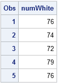
The following DATA step simulates five binomial trials. Each binomial trial represents 100 independent Bernoulli draws:

data Binom;
call streaminit(54321);
do i = 1 to 5;
   numWhite = rand("Binomial", 100, 0.75);  /* 100 draws; P(color=1) = 0.75 */
   output;
end;
run;
 
proc print; var numWhite; run;

Hypergeometric Trials

When sampling with replacement, the probability of choosing a white ball never changes. However, you can also sample without replacement. You start with N balls in the urn, of which K₁ are white. If you choose a white ball and remove it, the probability of choosing a white ball on the next draw is decreased. If you choose a black ball, the probability of choosing white increases. In addition, K₁ is an upper bound for the maximum number of white balls that can ever be drawn.

In spite of the changing probability, the distribution of the number of white balls when you sample without replacement is well understood. It is called the hypergeometric distribution. Like the binomial distribution, using the hypergeometric distribution saves time because you don't need to use the Bernoulli distribution (with a changing probability) to simulate drawing 100 balls without replacement.

The following DATA step uses the hypergeometric distribution to draw a sample of 100 balls from an urn that contains 120 balls, 90 of which are white. For this distribution it is necessary to specify three parameters: the total number of balls (N), and the initial number of white balls (K₁), and the sample size (n).

data Hyper;
call streaminit(54321);
do i = 1 to 5;
   /* sample without replacement from urn with 120 ball of which 90 are white */
   numWhite = rand("Hypergeometric", 120, 90, 100); /* N=120, K1=90; 100 draws */
   output;
end;
run;
 
proc print; var numWhite; run;

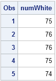
The values from the hypergeometric distribution have a smaller variance then the values from the binomial distribution. This is typical when the number of draws is close to the number of balls in the urn. When the number of balls is much greater than the number of draws, the hypergeometric distributions is similar to the binomial distribution.

In summary:

• Use the Bernoulli distribution to analyze the probability of pulling a colored ball from an urn with two colors.
• The binomial distribution model the distribution of the number of white balls when you sample n balls with replacement. In other words, you repeat n independent and identical Bernoulli trials.
• The hypergeometric distribution models the distribution of the number of white balls when you sample n balls without replacement.

Other related discrete probability distributions

There are other discrete probability functions that can model ball-and-urn experiments in which the question is "how many trials do you need until" some event occurs:

• The geometric distribution describes the number of trials that are needed to obtain one white ball. SAS supports the geometric distribution in the RAND function and in probability functions.
• The negative binomial distribution is the distribution of the number of black balls before a specified number of white balls are drawn in a sampling with replacement experiment. SAS supports the negative binomial distribution as well
• A lesser-known distribution is the negative hypergeometric distribution, which is the distribution of black balls when you sample without replacement. SAS does not support this distribution directly, but the hypergeometric distribution is useful for implementing it.