It is difficult to evaluate high-dimensional integrals. One numerical technique that can be useful is quasi-Monte Carlo integration. In this article, I show how you can generate quasirandom points in SAS and use them to evaluate a definite integral on a compact region. For simplicity, the example in this article integrates a function of two variables over a rectangular region.

What is quasi-Monte Carlo integration?

Multivariate calculus provides ways to integrate simple functions over simple 2-D and 3-D regions. However, analytical techniques often fail for high-dimensional regions and for complicated functions. Monte Carlo and quasi-Monte Carlo integration enables you to numerically estimate the definite integral of a function over an arbitrary high-dimensional region.

The standard Monte Carlo (MC) method evaluates a function at N points that are distributed uniformly at random in a region, then estimates the definite integral by using the average value of the function over those points. Previous articles show how to perform Monte Carlo integration in SAS for one-dimensional integrals and for two-dimensional integrals over rectangular and nonrectangular domains. For simplicity, this article discusses only rectangular regions.

The standard Monte Carlo method requires that you generate N points uniformly at random in the region. Unfortunately, Monte Carlo integration has slow convergence: The convergence is O(1/sqrt(N)). To halve the error, you must quadruple the number of points! This is because random points tend to have gaps and clusters, so some regions of the function's domain are sampled multiple times whereas other regions are sampled rarely.

In the quasi-Monte Carlo (QMC) method, you replace the pseudorandom points with quasirandom points. You evaluate the function at each point and compute the average value. As discussed in the Wikipedia article about quasi-Monte Carlo, the estimate of the integral converges according to O(1/N), which is much faster than for traditional Monte Carlo integration. This is because quasirandom points do not have gaps or clusters, which means the domain of the function is sampled more evenly.

The property of "no gaps or clusters" is accomplished by using deterministic low-discrepancy sequences to generate each coordinate of the points. This article generates quasirandom points by using the Halton sequence, but you can use other sequences. The Sobol sequences is one popular alternative.

The following sections use the SAS IML language to generate both pseudorandom and quasirandom points. The program compares the convergence for the MC and QMC methods for an integral of two variables on a rectangular domain.

Visualize pseudorandom and quasirandom points

A previous article shows how to create a library of SAS IML functions that generate quasirandom points by using Halton sequences. This deterministic sequence, derived from converting integers to different bases and reflecting the digits, produces points that fill the unit interval [0, 1] much more uniformly than pseudorandom numbers.

A GitHub repo contains all functions that generate the graphs and table in this article. You can run the program in the link to store the modules, then use the LOAD statement to use the functions in your own programs.

The following program compares pseudorandom and quasirandom points in a rectangular region in 2-D. In the DATA step, you can generate N uniform random variates in [0,1] by using the RAND("Uniform") function in a loop. In PROC IML, the RANDGEN subroutine enables you to generate many random variates in a single call. The variates on [0,1] can be transformed into any other interval [a,b] by using the affine transformation x → a + (b-a)*x. The following program generates N=1E4 points in the rectangle [0,π/2]x[0.1]:

proc iml;
N = 1E4;                 /* generate N points in D */
 
/* Domain of integration is D = [a,b] x [c,d] */
pi = constant('pi');
a = 0;  b = pi/2;          /* 0 < x < pi/2 */
c = 0;  d = 1;             /* 0 < y < 1    */
x0 = a || c;               /* offset vector */
s = (b-a) || (d-c);        /* scaling vector */
 
title "Pseudorandom Evaluation Points";
call randseed(1234);
X = j(N,2);                      
call randgen(X, "uniform", 0, 1);  /* X ~ U[0,1]^2 */
X = x0 + s # X;                    /* X ~ U(D) */
call scatter(X[,1], X[,2]) grid={x y} 
     option="markerattrs=(symbol=circlefilled size=3) transparency=0.5";

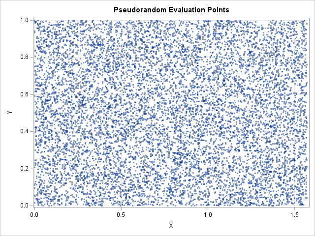
The scatter plot shows the gaps and clusters that are typical of points that are distributed uniformly at random. If you evaluate a function at these points, the function is sampled more often in some regions than in other regions.

Let's compare this situation to a quasirandom set of points. The following statements load the Halton functions, then generate 1E4 quasirandom points. Be sure to run the program mentioned in the Appendix to store the functions. The call to QRand_Halton(N,2) generates an Nx2 matrix, Q, where each row of Q is a quasirandom point in the unit square [0.1]x[0,1].

load module=_ALL_;    /* first run the program in the Appendix to store the Halton and quasirandom functions */
 
title "Quasirandom Evaluation Points";
Q = QRand_Halton(N, 2);            /* Q is quasirandom in unit square */
Q = x0 + s # Q;                    /* Q is quasirandom in D */
call scatter(Q[,1], Q[,2]) grid={x y} 
     option="markerattrs=(symbol=circlefilled size=3) transparency=0.5";

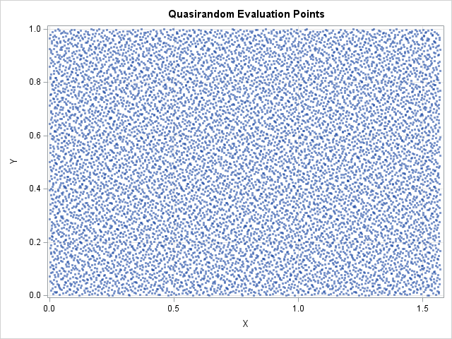
The scatter plot of the quasirandom points shows no gaps or clusters. Because of the way a Halton sequence is constructed, each new point is generated in an empty space among the previous set of points. As you add more and more points from the Halton sequence, the empty regions get smaller and smaller.

You could achieve a "no gaps, no clusters" point pattern by using points on a regular grid, but the grid method lacks an important feature of the low-discrepancy sequences. Namely, in a low-discrepancy sequence, a sequence of length N contains all the points of the sequence of length N-1, plus one additional point. A regular-spaced grid does not have that property. For example, a set of nine evenly spaced points in [0,1] is 1/10, 2/10, ..., 9/10. But none of these points are contained in the set of eight evenly spaced points, which is 1/9, 2/9, ..., 8/9. In integration, you must evaluate a function at every point of a quasi-random point set. A low-discrepancy sequence enables you to generate points sequentially and monitor the convergence of the integral. You can generate points until the integral converges and then stop.

Monte Carlo and quasi-Monte Carlo Integration

A previous article shows how to estimate the definite integral of a function of two variables by using the traditional Monte Carlo integration in SAS. In that article, the function is f(x,y) = cos(x)*exp(y), and the domain of integration is D = [0,π/2]x[0,1]. The previous section generated both pseudorandom points (X) and quasirandom points (Q) in this domain. To estimate the integral, you evaluate the function on the set of points, take the average, and scale the average to account for the area of the domain. The following statements estimate the integral first by using the pseudorandom points and next by using the quasirandom points.

/***********************************************/
/* estimate the double integral in https://blogs.sas.com/content/iml/2021/04/07/double-integral-monte-carlo.html */
/***********************************************/
/* define integrand: f(x,y) = cos(x)*exp(y) */
start func(x);
   return cos(x[,1]) # exp(x[,2]);
finish;
 
/* the double integral is separable; solve exactly */
Exact = (sin(b)-sin(a))*(exp(d)-exp(c));  
Area = (b-a)*(d-c);                /* area of rectangular region */
 
/* MC = Monte Carlo */
W = func(X);                       /* f(X1,X2) for columns of X */
MCEst = Area * mean(W);            /* MC estimate of double integral */
DiffMC = Exact - MCEst;
/* QMC = quasi-Monte Carlo */
W = func(Q);                       /* f(Q1,Q2) for columns of Q */
QMCEst = Area * mean(W);           /* MC estimate of double integral */
DiffQMC = Exact - QMCEst;
print Exact MCEst QMCEst DiffMC DiffQMC;

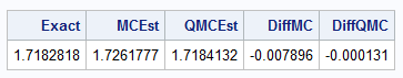
I chose this function because the definite integral has an analytical solution. On the domain, the exact integral is e – 1 ≈ 1.71828. With this random number seed, the traditional Monte Carlo estimate is accurate to about 0.5% of the true value with N=10,000 points. The first wrong digit is in the second decimal place. In contrast, the quasi-Monte Carlo estimate is accurate to about 0.008% with the same number of points. The first wrong digit is in the fourth decimal place.

The fact that the Monte Carlo estimate depends on the random number seed can be annoying. It introduces random variation into the estimate. It makes the estimate hard to reproduce for users of other software. It means that the Monte Carlo estimate has a large standard error. In contrast, there is nothing random about the quasi-Monte Carlo estimate. Any other implementation that uses Halton sequences and the same choice for Halton bases will produce exactly the same estimate.

The convergence of MC and QMC integration

Let's take a closer look at the convergence of the integral estimates for both the MC and QMC methods. As I have discussed previously, the convergence for the traditional MC method is fairly slow, and there is considerable variation in the estimate. The estimate for the QMC method is much tamer. The following statements show the convergence by plotting the estimate of the integral for N=100, 200, ..., 10000 points.

/* How does the estimate depend on the sample size? 
   We have already computed W = func(X) */
size = do(1E2, N, 1E2);
QMCest = j(1,ncol(size),.);
do i = 1 to ncol(size);
   Y = W[1:size[i],];              /* Y = f(Q) for the first size[i] points */
   QMCEst[i] = Area*mean(Y);       /* estimate integral */
end;
 
title "Quasi-Monte Carlo Estimates as a Function of Sample Size";
stmt = "refline " + char(Exact,6,4) + "/ axis=y; format size comma10.;";
call scatter(size, QMCEst) grid={x y} other=stmt label={"Sample Size"};

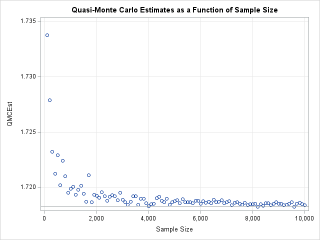
The scatter plot shows the convergence of the estimate for the integral as N increases. You can see that the estimate converges quickly. The estimate is already good after using only 2,000 quasirandom points. The estimate generally improves as N increases, and there are no wild swings in the estimate as can happen with the traditional Monte Carlo method. As a rule of thumb, QMC enables you to use fewer points than MC to achieve the same accuracy. For that reason, the QMC is often preferred over MC for estimating definite integrals in low to moderate dimensions (such as d ≤ 10).

Summary

This article demonstrates quasi-Monte Carlo integration in SAS by using SAS IML functions that implement Halton sequences. An example of a 2-D integral shows that the QMC estimate converges quickly. The traditional MC converges like O(1/sqrt(N)), whereas the QMC estimate converges as O(1/N). In addition, QMC is deterministic, which means that the answer does not depend on a random number seed.

Before concluding, I mention two drawbacks of the quasi-Monte Carlo method. First, not every integral of interest has a finite domain. There are plenty of integrals in probability theory that require integration over an infinite domain. Second, in this implementation, I use consecutive prime numbers (2, 3, 5, ...) as the bases to generate a Halton sequence in each coordinate direction. This technique works well for small primes, so quasi-Monte Carlo integration with Halton sequence is often used for six or fewer dimensions. It is known that for larger primes (for example, 17 and 19), the Halton sequences might be strongly correlated. The Wikipedia article mentions some ways to overcome this deficiency.

Appendix: SAS IML functions for generating quasirandom numbers in d dimensions

The SAS IML functions that are used to create all graphs and table in this article are available on GitHub. They enable you to generate quasirandom ordered tuplets up to d=168 dimensions. Almost all of the functions are explained and demonstrated in previous article about how to generate a Halton sequence. The two new functions are

• HaltonSeqD : Create a matrix with N rows where each column is a Halton sequence for a specified base
• QRand_Halton : Create a matrix with N rows and d columns, where each column is a Halton sequence for a base chosen from the first d prime numbers: 2, 3, 5, 7, 11, ...