A previous article discusses Welford's one-pass method for computing the sample mean and variance. The article mentions that a useful application of Welford's formulas is to monitor the convergence of a Monte Carlo simulation. This article shows how to implement that strategy in SAS.
The Goldilocks Principle for Monte Carlo methods
The Goldilocks Principle is a name given to efforts to achieve a balance between extremes. For example, suppose my goal is to ensure that my house is clean. There are two extremes. If I spend every hour of every weekend cleaning, dusting, and vacuuming, my house will look pristine. However, I expend a lot of time and effort. In contrast, if I spend no time cleaning, the house will be dirty. Somewhere between those two extremes is the Goldilocks strategy: I exert enough effort to make the house look nice, but the effort doesn't consume all my resources. The optimal amount of effort depends on how clean I want the house to be.
The same trade-offs apply in many areas of computational statistics. In Monte Carlo simulations, you can get better estimates if you run more simulations, but more simulations require more time and computing resources. A traditional Monte Carlo simulation looks like this:
- Choose the number of simulations, B, that you plan to run. This is essentially a GUESS!
- Generate a random sample of size N and compute statistics for that sample.
- Repeat this B times. Store all sample statistics in an array.
- Compute the Monte Carlo mean and report a measure of accuracy, such as the standard error or a confidence interval.
The problem is we do not know a priori how large to choose B. If B is too small, the simulation study is underpowered, and the final Monte Carlo estimate is not very accurate. Consequently, you might need to repeat the simulation with a larger value of B to obtain a more accurate estimate. On the other hand, if B is too large, the Monte Carlo estimate is very accurate, but you wasted time and CPU costs needlessly.
By using Welford's update formula inside a simulation loop, you don't have to guess a value for B, number of Monte Carlo simulations. Instead, you treat the statistic from each random sample as a piece of streaming data. You keep track of the mean and variance of the Monte Carlo estimate. When a confidence interval for the estimate is sufficiently small, you stop the simulation loop. This is sometimes called an adaptive Monte Carlo simulation.
Example of the traditional Monte Carlo simulation in SAS
Before looking at the adaptive Monte Carlo method, let's run a traditional simulation study. Suppose you have data (N=100) that you believe to be exponentially distributed. You compute the mean of the sample to estimate the population mean. A classic problem in statistics is to infer how close the estimate is to the true population mean. To do that, you need to understand the sampling distribution of the mean in a random exponential sample of size N=100. There are several ways to do that, but I want to use a Monte Carlo simulation.
The following Monte Carlo simulation uses PROC IML to generate B=10,000 random samples from the Expo(λ=10) distribution, where λ is a scale parameter. The program computes the sample mean for each random sample. It then computes the Monte Carlo estimate of the statistic by taking the mean of the 10,000 samples statistics. Lastly, it estimates the standard error of the Monte Carlo estimate and uses that to form a 99.7% confidence interval for the estimate.
/* traditional Monte Carlo simulation: Compute the Monte Carlo estimate of the mean of a random sample of size N. Do this a large number of times (B) to ensure that the estimate is accurate. For this example, we sample from the Exp(lambda) distribution where lambda=10 is a scale parameter. The true mean is lambda. */ proc iml; call randseed(1234); N = 100; /* sample size */ B = 10000; /* number of Monte Carlo samples */ lambda = 10; /* scale parameter for Expo distrib */ sample_mean = j(B,1,.); x = j(N,1); do i = 1 to B; call randgen(x, "Expo", lambda); sample_mean[i] = mean(x); end; MC_est = mean(sample_mean); /* MC estimate of statistic */ SE_est = std(sample_mean) / sqrt(B); /* MC standard error */ width = 3*SE_est; /* half-width of CI: 3*SE ==> 99.7% CI */ Lower_CL = MC_est - width; Upper_CL = MC_est + width; print MC_est SE_est width Lower_CL Upper_CL; /* we saved all the Monte Carlo estimates, so plot the sampling distribution */ title "MC Distribution"; title2 "N=100; B=10,000"; call histogram(sample_mean) other="refline 9.9860983 9.9560683 10.016128/axis=x;"; |
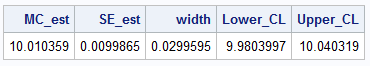
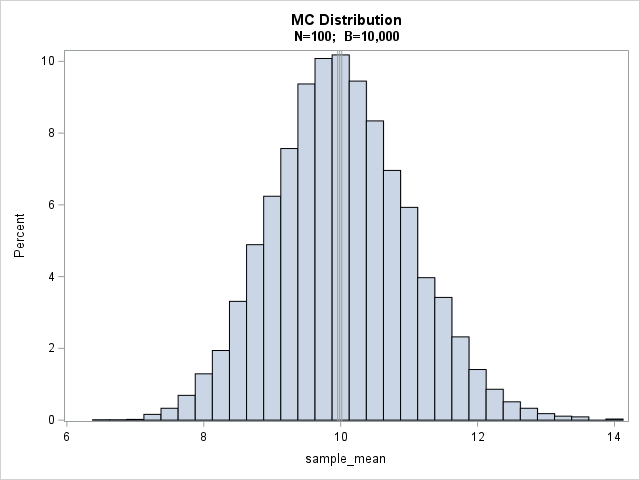
What do we learn from this output about the accuracy of the Monte Carlo estimate? First, the histogram shows that the sample mean in random samples of size N=100 is quite variable, but approximately normally distributed. The Monte Carlo estimate of the population mean is the average of all these sample values. The Monte Carlo estimate and a 99.7% confidence interval are overlaid on the histogram. After B=10,000 simulations, a 99.7% confidence interval for the Monte Carlo estimate has a half-width of about 0.03.
If we want the Monte Carlo estimate to be more accurate, we can run additional simulations. How many simulations would we need for the 99.7% CI to have a half-width of 0.01 units? Theory tells us that the Monte Carlo standard error is proportional to 1/sqrt(B). The standard interpretation of this result is that if you want to cut the standard error in half, you must quadruple the number of simulations. In this case, we want to reduce the standard error from 0.03 to 0.01 (a ratio of 1/3), so we expect this to happen if we perform 9 times as many simulations, or roughly B=90,000.
These calculations are based on having run an initial simulation study with low power. This is often a good idea. But if you monitor the standard error during the simulation loop, you might not need the initial study. Instead, you can keep iterating until a confidence interval for the standard error is below some pre-determined tolerance.
Adaptive Monte Carlo simulation in SAS
This section implements an adaptive Monte Carlo simulation in SAS IML. The main difference between an adaptive program and a standard Monte Carlo simulation is that the adaptive program uses a DO-UNTIL statement to repeat the trials until a confidence interval for the estimate is sufficiently small.
In the previous example, the accuracy of the MC estimate after 10,000 iterations is about 0.03, as estimated by the half-width of a 99.7% confidence interval. Instead of running the entire simulation and then checking the accuracy at the end, you can use Welford's formula to provide a running standard error. You can use DO-UNTIL logic to loop until the Monte Carlo estimate is sufficiently accurate
The following IML program implements this adaptive method. Inside the iteration loop, Welford's formula updates the mean and variance. The program always generates at least 1,000 random samples (minB) but never computes more than 100,000 samples (maxB).
/* Adaptive Monte Carlo simulation using Welford's formula */ proc iml; call randseed(1234); N = 100; /* sample size */ maxB = 100000; /* maximum number of Monte Carlo samples */ minB = 1000; /* run at least this many trials */ lambda = 10; /* scale parameter for Expo distrib */ x = j(N,1); m = 0; varsum = 0; /* Welford's running totals */ tol = 0.01; /* desired accuracy */ err = 2*tol; /* make sure err > tol to enter loop */ do k = 1 to maxB until(err < tol); /* you can put ANY simulation here */ call randgen(x, "Expo", lambda); y = mean(x); /* use Welford's online mean and variance formulas to monitor convergence */ varsum = varsum + (k-1) * (y - m)**2 / k; /* update the sum of squared differences */ m = m + (y - m) / k; /* update the mean */ if k > minB then do; sd = sqrt(varsum/(k-1)); err = 3*sd / sqrt(k); /* 3*SE ==> 99.7% confidence */ end; end; print k m err[L='error']; quit; |
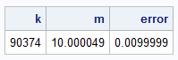
By using Welford's streaming mean and variance formulas inside the DO-UNTIL loop, the simulation runs for exactly as long as required. When the tolerance is 0.01, the simulation (for this random-number seed) generates 90,374 samples. This is an amazingly close agreement with the theoretical estimate, which predicted 90,000 samples.
Summary
This article shows a modern application of Welford's formulas for the streaming mean and variance of data. The application is to iterate an algorithm until the accuracy of an estimate is less than some specified tolerance. Here, the algorithm is a Monte Carlo simulation, and the estimate is the Monte Carlo estimate of a sample mean.
I recently used this approach while computing the Monte Carlo approximation of an integral. I wanted to ensure that my integral estimate was accurate to within a certain tolerance. By monitoring the estimate and its standard error, I was able to guarantee the accuracy of the integral calculation.
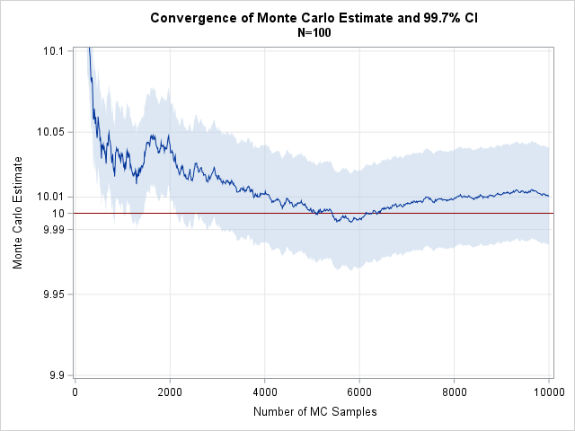
Appendix: The width of the confidence interval
I didn't want this article to be too long, but I wanted to show a graph of the running Monte Carlo estimate and its 99.7% confidence interval. The Monte Carlo estimate converges quickly, as shown in the graph below. However, the estimate bounces around. You can see that when B=5000, the MC estimate is very close to the population mean, which is 10. However, the confidence interval for the estimate (shown by the gray-blue band) has a half-width of about 0.025. Indeed, as we add more simulations, the MC estimate jitters up and down, so we cannot say with confidence that we have an accurate estimate. Eventually, when B exceeds 90,000, not only is the estimate close to the value 10, but the gray-blue band has a half-width less than 0.01.