On the evaluation of the function exp(x) - 1

Recently I wrote about numerical analysis problem: the accurate computation of log(1+x) when x is close to 0. A naive computation of log(1+x) loses accuracy if you call the LOG function, which is why the SAS language provides the built-in LOG1PX for this computation. In addition, I showed that you can use numerical methods to implement an accurate evaluation of that function if your computer software does not have a built-in function.

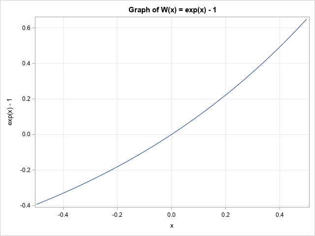
There are similar quantities that also lose precision if you evaluate them naively. One of these is the inverse function for log(1+x), which is the function W(x) = exp(x) – 1. The graph of this function is shown to the right. To the casual observer, the function appears to be well-behaved near x=0. And it is, mathematically. Numerically, however, you must be careful evaluating W(x) when x is very small such as |x| ≤ 1E-13). This situation comes up in financial applications, as well as in probability and statistics.

This article shows three methods for evaluating exp(x) – 1 accurately when x is near 0. Some of the ideas in this article are from the excellent article Beebe, N. H. F., (2002) "Computation of expm1(x) = exp(x) - 1." See Beebe (2002) for a careful numerical analysis of this problem.

SAS supports the EXPM1 function as of the 23.11 Release of SAS Viya. If you are using SAS 9 or an earlier version of SAS Viya, you can use the formulas in this article to implement the EXPM1 function yourself.

Understanding the problem

When x is near 0, exp(x) is close to 1. It turns out that a naive evaluation of W(x) = exp(x) – 1 by calling the EXP function results in a loss of accuracy due to "catastrophic cancellation" when 1 is subtracted from exp(x). This is shown in the following SAS DATA step. The fact that W(x) and log1px(x) are inverses means that log1px(W(x)) should be very close to x for all values of x. We can use that fact (or the other inverse function, W(log1px(x))) to test the accuracy of the computation of W(x).

/* straightforward evaluation by using EXP function. This method starts to lose accuracy for x < 0.4 */ 
data Expm1Naive;
do pow = -10 to -17 by -1;
   x = 10**pow;
   Naive = exp(x) - 1;
 
   /* apply the inverse; y=x in exact arithmetic */
   x2 = log1px( Naive ); 
   RelError = (x-x2)/x;
   output;
end;
drop pow;
run;
 
proc print noobs;
   format Naive E18.;
   var x Naive x2 RelError;
run;

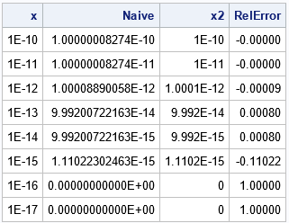
The table shows values of exp(x) – 1 for several small, positive, values of x. For x ≤ 1E-15, the naive calculation returns 0 because exp(x) and x have cancelled each other to machine precision. If you look only at the NAIVE column, the cancellation seems abrupt. However, if you apply the inverse function and look at the relative error between x and log1px(W(x)), you can see that the relative error gets larger and larger as x gets smaller and smaller.

This shows that the naive computation of exp(x) – 1 (that is, by calling the EXP function) is not accurate when x is very small. The next sections describe alternative computations that are more accurate.

A Taylor series approximation

You can look at the Taylor series near x=0 to understand what is happening and how to fix it. The Taylor series for exp(x) is well known:
exp(x) = 1 + x + x²/2! + x³/3! + x⁴/4! + x⁵/5! + ...
We want to compute exp(x) – 1, so cancel the 1 and factor out an x to get
exp(x) – 1 = x*[ 1 + x/2! + x²/3! + x⁵/4! + x⁴/5! + ... ]

It is useful to think of the infinite series in brackets as the Taylor series for the function Q(x) = (exp(x)-1)/x, which has a removeable singularity at x=0. A stable method for approximating W(x) is to compute it as x*Q(x) for various approximations of Q(x). For example, the following DATA step uses a 6-term Taylor series approximation of Q(x). The Taylor polynomial is evaluated by using Horner's method:

/* use exp(x)-1 for abs(x) > 0.1. For smaller values, use numerical approximation */
data Expm1Taylor;
do pow = -10 to -17 by -1;
   x = 10**pow;
   /* approximate by using a 6-term Taylor polynomial */
   QTaylor = 1 + x/2*(1 + x/3*(1 + x/4*(1 + x/5*(1 + x/6))));
   Taylor  = x*QTaylor;
 
   /* these are inverse functions, so y=x in exact arithmetic */
   x2 = log1px( Taylor ); 
   RelError = (x-x2)/x;
   output;
end;
drop pow;
run;
 
proc print noobs;
   format Taylor E18.;
   var x Taylor x2 RelError;
run;

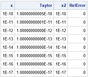
The table shows that the Taylor series approximation is a perfect inverse to the LOG1PX function for the specified values. For larger values of x, the Taylor polynomial will deviate from W(x).

A rational function approximation

There are many ways to approximate the quantity Q(x) by using a rational function, which is a ratio of low-order polynomials. Beebe (2002) uses the ratio of a quadratic polynomial and a cubic polynomial, although many other choices are possible. The following rational function approximation is used by R, which is an open-source statistical software package.

/* use exp(x)-1 for abs(x) > 0.1. For smaller values, use numerical approximation */
/* rational function approximation used by R */
data Expm1RatFunc;
do pow = -10 to -17 by -1;
   x = 10**pow;
   numerPoly = 
    1.0 +
   (9.14041914819518e-10 +
    0.0238082361044469 * x) * x;
   denomPoly =
    1.0 +
    (-0.499999999085958 +
    ( 0.107141568980644 +
    (-0.0119041179760821 + 
     0.95130811860248e-4 * x) * x) * x) * x;
   QRatFunc = numerPoly / denomPoly;
   RatFunc = x*QRatFunc;
 
   /* these are inverse functions, so y=x in exact arithmetic */
   x2 = log1px( RatFunc ); 
   RelError = (x-x2)/x;
   output;
end;
drop pow numerPoly denomPoly;
run;
 
proc print noobs;
   format RatFunc E18.;
   var x RatFunc x2 RelError;
run;

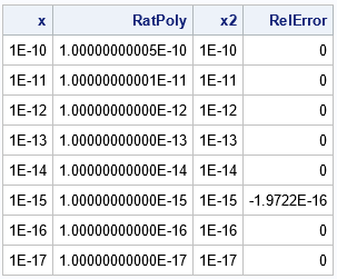
The table shows that the rational function approximation is accurate for the specified values of x.

Computation in software

SAS supports the EXPM1 function, evaluates exp(x) – 1, as of the 23.11 Release of SAS Viya. If you are using SAS 9 or an earlier version of SAS Viya, you can use the methods in this article to define a user-defined FCMP function or to define a SAS IML module. You would evaluate exp(x) – 1 directly when |x| is larger than some cutoff (for example, 0.1) and use an approximation when x is very small.

Other software packages that provide an "expm1" function include the following:

In MATLAB, use the expm1 function.
In Python, import the NumPy module and use the numpy.expm1 function.
In R, use the expm1 function.

Summary

The expression exp(x) – 1 is easy to evaluate when x is bounded away from 0, but can lose accuracy when x is close to 0. This article shows two ways to evaluate the expression exp(x) – 1 accurately when x is close to 0. You can use a Taylor polynomial or a rational function to accurately evaluate the expression for tiny values of x in software that does not support a built-in version of the "expm1" function. For more details, see Beebe (2002)

Blogs