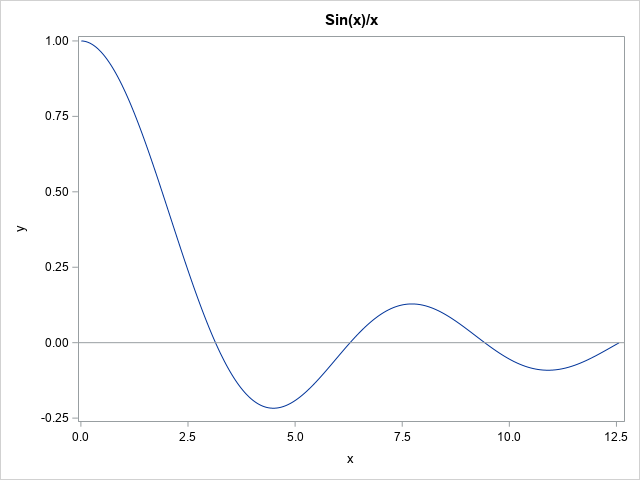
The other day I was trying to numerically integrate the function f(x) = sin(x)/x on the domain [0,∞). The graph of this function is shown to the right. In SAS, you can use the QUAD subroutine in SAS IML software to perform numerical integration. Some numerical integrators have difficulty computing this integral because (1) it on an infinite domain, and (2) the integrand is undefined at x=0. This article focuses on the latter issue and describes a standard way to adjust a difficult-to-evaluate function by using a Taylor series approximation to the function.

The Taylor series for sin(x)/x

Students of calculus might remember that the function sin(x)/x has a removable singularity at x=0. The limit as x → 0 of f(x) is 1, so you can define a new function sinc(x) which is f(x) when x ≠ 0 and 1 when x=0. The sinc function is continuous and has no singularities.

For this function, removing the singularity at x=0 is a simple way to handle the issue. However, for more complicated functions, there might be an interval near x=0 on which you cannot numerically evaluate the function. In these cases, you can often approximate the function on the interval by using the Taylor series truncation of the function.

For example, the sine function near x=0 has the Taylor series representation
    sin(x) = x – x³/3! + x⁵/5! – ...
If you divide each term in the series by x, then the sinc function near x=0 can be approximated by using the first two terms of the resulting series, which is
    sinc(x) ≈ 1 – x²/6

Use the Taylor series to avoid hard-to-evaluate intervals

The following SAS DATA step uses this representation when x < C for a small value of C. In practice, you might choose C = 0.1 or smaller, but I will choose a larger value of C so that we can more easily zoom in and see what the function looks like near x=C. For this example, I choose C = 0.2.

%let C = 0.2;   /* cutoff; in practice, C would be MUCH smaller */
data Sinc2;
C = &C;      
keep x y;
dx = 0.001;
do x = 0 to 2*C by dx;
   if x < C then 
      y = 1 - x**2/6; 
   else 
      y = sin(x) / x;
   output;
end;
run;
 
title "Approximation to Sin(x)/x Near x=0";
proc sgplot data=Sinc2;
   series x=x y=y;
   refline &C / axis=x;
run;

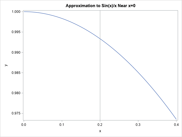
The plot shows the graph of function which is defined by using a Taylor series truncation to the left of C=0.2 and the sin(x)/x function to the right. At this scale, the function looks continuous, but it isn't. The next image zooms in on the graph near x=C:

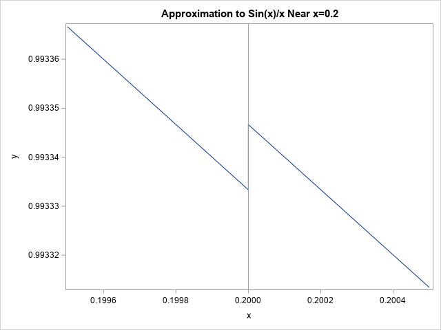
Now you can see that there is a gap at x=C. The gap has the value sin(C) / C – (1 – C²/6) ≈ 1.33E-5. You can use math to show that the error will be less than |C⁴/120| for any value of C. (That expression is the next term in the alternating Taylor series.)

You can make the gap smaller by choosing a smaller value of C or by keeping additional terms in the Taylor series, but the gap never goes away.

A cautionary tale

Although using a Taylor series can be a valuable tool to avoid singularities and numerical difficulties near singularities, the previous serves to remind us that the resulting graph is not usually continuous. This has implications in numerical computations. For example, if you are integrating the function on [0,b], you should break up the integral and perform two integrals: one on [0,C] and the other on [C,b]. This prevents you from attempting to integrate across the point of discontinuity, which is usually unwise. Similarly, if you are using this function as an objective function in an optimization, the solver might encounter difficulties near x=C where the function is discontinuous.

There are ways to adjust the Taylor series so that you get continuity at x=C, but I will leave that discussion for another day.

Summary

If a function has an interval on which the function is difficult to evaluate, you can often replace the function on the interval by using a Taylor series approximation. In many cases, you can choose a value x=C and define a new function by using a Taylor series truncation on one side of x=C and by using the original function on the other side. However, it is important to realize that the resulting function is not continuous at x=C, so you must exercise care when performing numerical computations on intervals that contain C.