In SAS, you can approximate the exponential of a matrix by using the EXPMATRIX function in SAS IML software. This article discusses the exponential of a matrix: what it is, how to compute it, why it is useful, and why you should think of it as a linear map that converts a continuous system of differential equations into a discrete iterative process.

What is the matrix exponential?

The matrix exponential function is a mapping from the set of square matrices to the set of invertible matrices. (Actually, these sets are non-commutative rings since they support addition and multiplication.) The matrix exponential function is a generalization of the familiar exponential function. Denote the matrix exponential function by expm(·). For a square matrix, A, the matrix expm(A) is defined by the following infinite series, which is based on the Taylor series expansion for the scalar exponential function:
$\mathrm{expm}(A) = I + A + \frac{A^2}{2!} + \frac{A^3}{3!} + \cdots$

The infinite series converges for all square matrices. Interestingly, just as the function exp: R → R sends an arbitrary number to a positive number, the expm function maps an arbitrary square matrix to an invertible matrix. That is, if A is any square matrix, then the matrix B = expm(A) is invertible.

The matrix exponential is often encountered in an elementary course on ordinary differential equations. If x is a vector and A is an n x n constant matrix, then the linear homogeneous differential equation with constant coefficients x' = A x has a solution that is concisely written as x(t) = expm(t*A) x₀, where x₀ is the initial state of the system at t=0. When I was taught the matrix exponential, I thought it was merely a notational convenience. But, as I show in this article, it is much more.

If you are not familiar with the matrix exponential, the following references provide some background:

• The Wikipedia article on "Matrix Exponential."
• Nick Higham's (2020) introductory article, "What Is the Matrix Exponential?"
• Section 11.4, "Matrix Exponential," in Gustafson, G., "Differential Equations and Linear Algebra" online textbook (accessed 30Apr2023).

How to compute the matrix exponential?

Many elementary textbooks use the definition of the expm function to compute expm(A) for certain types of matrices. For example, if A is a diagonal matrix, then expm(A) is simply the diagonal matrix B whose diagonal element B_ii is equal to exp(A_ii). Another easy computation is for nilpotent matrices, since then the infinite series becomes finite.

In general, it is not easy to numerically compute the exponential of a general matrix. Moler and Van Loan (198=78, revised 2003) published a famous paper titled "Nineteen Dubious Ways to Compute the Exponential of a Matrix." The SAS IML computation uses a scaled Padé approximation, which is presented in Golub and Van Loan (Matrix Computations, 1996, 3rd Ed, p. 572-574).

In applications, we are often interested in the matrix expm(t*A), where t > 0, which is the general solution of the differential equation x' = A x at time t. Since a diagonal matrix is most understandable, the following call to PROC IML computes the matrix exponential for a diagonal matrix at t=2. It then compares the computation to the exact value, which is also a diagonal matrix:

proc iml;
/* let's use two matrices from ODEs */
t = 2;
D = {-1 0,
      0 0.5};
ExpmD_2 = ExpMatrix(t*D);    /* expm(2*D) */
Print ExpmD_2[L="expm(2*D)"];
 
/* The diagonal elements of D are -1 and 0.5. The matrix exponential for t*D is equal to 
   expm(t*D) = [ exp(-1*t)   0          ]
               [ 0           exp(0.5*t) ]
*/
Exact = ( exp(-t) || 0          ) //
        ( 0       || exp(0.5*t) );
maxDiff = max(abs(ExpmD_2 - Exact));
print maxDiff;

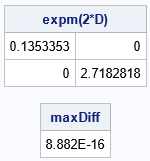
The output shows that, to machine precision, the EXPMATRIX function returns the exact value of the matrix exponential.

The geometric interpretation of the matrix exponential

Most textbooks use the matrix exponential as a shorthand notation for the general solution of a system of first-order ODEs with constant coefficients. But it is more than that! The matrix exponential converts a continuous-time system (the ODE) into a discrete-time system. If x(t0) is the state of the system at time t0, you can obtain the state of the system at time t1 by matrix multiplication: x(t1) = expm(dt*A)*x(t0), where dt = t1 - t0. In other words, the matrix exponential (B = expm(dt*A)) enables you to map the state forward (or backward!) in time by performing a matrix multiplication!

This is useful because we often want to find the solution of an ODE at a discrete set of time points, such as t = 0.1, 0.2, 0.3, and so forth. For example, suppose you want the solution of a linear ODE that starts in the state x0. One way to compute the trajectory from that initial state is to compute a sequence of matrix exponentials such as expm(0.1*A), expm(0.2*A), expm(0.3*A), and so forth. You can use these matrices to transform the initial state to the state of the system:
     x1 = expm(0.1*A)*x0
     x2 = expm(0.2*A)*x0
     x3 = expm(0.3*A)*x0
     ...

However, the preceding computation is not efficient. There is no need to compute a large number of exponential matrices of the form expm(t*A) for different t values. Instead, you only need to compute ONE matrix, which is B = expm(0.1*A). You can then use matrix multiplication to iterate the trajectory forward in time from the initial state:
     x1 = B*x0
     x2 = B*x1
     x3 = B*x2
     ...

In PROC IML, the computation looks like this:

proc iml;
/* more efficient: Let B be the mapping that moves the solution 
   ahead by dt = 0.1. Thus, the continuous integration is transformed
   into a discrete mapping from x(t) to x(t+dt).
   You can iterate to get the solutions at a sequence of times,*/
A = {-1 0,            /* matrix of linear coefficients */
      0 0.5};
dt = 0.1;             /* time increment */
B = ExpMatrix(dt*A);  /* map any state to new state, which is dt time units in future */
x0 = {1.0, 0.4};      /* x0 is initial state */
 
numT = 20;
time = T( do(0, numT*dt, dt) );   /* vector of time points */
Soln = j(numT, 2, .);             /* allocate space for trajectory */
Soln[1,] = T( x0 );               /* start trajectory at x0 */
xt = x0;
/* iterative method */
do i = 2 to numT;
  xt = B * xt;                    /* compute solution at next time point */
  Soln[i, ] = T( xt );
end;

The solution is computed at t=0.1, 0.2, ..., 2.0. Notice that only matrix multiplication is used. The matrix is the "map-the-state-forward matrix," which is computed by using the matrix exponential, B. The matrix B maps each state at time t to the next state at time t + dt. Notice that this is not an approximate solution. It is an exact solution at each time point.

You can graph the trajectories versus time to verify that the first component is exponentially decaying and the second component is exponentially growing:

create LinearSoln from time Soln[c={'time' 'x' 'y'}];
append from time Soln;
close;
 
submit;
title "Solution of Linear ODE";
title2 "(x(0), y(0)) = (1.0, 0.4)";
proc sgplot data=LinearSoln;
   series x=time y=x / curvelabel;
   series x=time y=y / curvelabel;
   xaxis values=(0 to 2 by 0.5) minor minorcount=4 grid;
   yaxis grid;
run;
endsubmit;

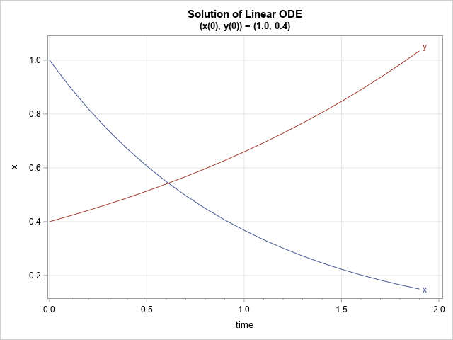
Because the original linear system is diagonal, it is easy to write down the formulas for the exact solution. The first component has the solution x(t) = exp(-t), and the second component has the solution y(t) = 0.4 exp(0.5*t). This agrees with the graph.

The matrix exponential can draw vector fields

Did you know that the matrix exponential can be used to draw a representation of the underlying vector field? Furthermore, the matrix exponential enables you to vectorize the computation. You can compute the entire vector field by using a single matrix multiplication. To visualize the vector field, do the following:

1. Create a grid of (x,y) positions at which you want to visualize the linear vector field given by A.
2. Use the matrix exponential to create a matrix that maps each state forward in time by a small amount. For example, the following program uses B = expm(0.1*A) to map each point forward by 0.1 time units.

/* draw a vector field for the linear system x`=A*x */
x0 = expandgrid( do(-1,1,0.2), do(-1,1,0.2) );
v  = B*x0`;    /* map each state forward by 0.1 units of time */
x1 = v`;       /* transpose to get (x_final, y_final) */
 
create VF from x0 x1[c={'x0' 'y0' 'x1' 'y1'}];
   append from x0 x1;
close;
 
submit;
title "Vector Field for Linear System";
proc sgplot data=VF aspect=1;
   vector x=x1 y=y1 / xorigin=x0 yorigin=y0;
   xaxis grid;
   yaxis grid;
run;
endsubmit;

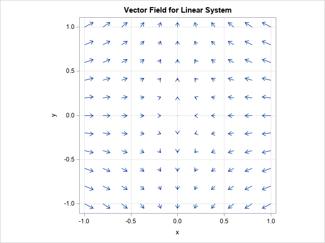
The graph visualizes the linear vector field. The origin is a fixed point. Trajectories approach the origin along the X axis and move away from the origin along the Y axis. Notice that the entire graph is produced by using one matrix multiplication; there are no loops.

Summary

This article discusses the matrix exponential operator. In elementary courses on differential equations, it is often presented either as a formal power series of matrices or as a concise notation that represents the general solution of a linear system of ODEs. This article demonstrates two useful properties of the matrix exponential. First, it can be used as a "one-step" operator that enables you to generate points along a trajectory by iterating an initial state. Thus, the matrix exponential converts a continuous-time system into a discrete iterative system. Second, it can efficiently visualize a vector field by iterating a grid of initial states forward in time and using arrows to connect the initial and final states.