Estimate the pth root of a Markov transition matrix

You can use a Markov transition matrix to model the transition of an entity between a set of discrete states. A transition matrix is also called a stochastic matrix. A previous article describes how to use transition matrices for stochastic modeling.

You can estimate a Markov transition matrix by using historical data that is collected over a certain length of time. Let's say that you are interested in the transitions of working-age individuals between three employment states: employed full-time, employed part-time, and unemployed. You survey a set of individuals and ask them to report their employment status today and one year ago. You can use their answers to estimate the annual transition matrix between the three employment states.

But suppose you want to estimate the MONTHLY transition matrix from the data. That is, what is the average monthly rate at which workers transition between the three states of employment? To answer that question, you need to compute the 12th root of the transition matrix. That is, if T is the annual transition matrix, you want to find another transition matrix, M, such that M¹² = T. Unfortunately, this is not always possible. Not all matrices have pth roots, and a pth root (if it exists) is not necessarily a transition matrix. In an interesting paper, Higham and Lin ("On pth roots of stochastic matrices", 2011) characterize when a real matrix has a real pth root and when the pth root of a transition matrix is itself a transition matrix.

Since an exact solution is not always possible, you can relax the requirement of equality and instead find a transition matrix, M, such that M¹² is as close as possible to T in the least squares sense. Given a transition matrix, T, this article shows how to use nonlinear optimization in SAS to compute a transition matrix, M, that is approximately the pth root of T. To keep the exposition simple, I use p=12, but the algorithm works equally well for other values of p.

A Markov transition matrix

To begin investigating the pth root of a transition matrix, let's first use the following 3 x 3 annual transition matrix:

    [ 0.8  0.1  0.1  ]
T = [ 0.25 0.6  0.15 ]
    [ 0.25 0.25 0.5  ]

The (i,j)th entry is the probability of transitioning from State i to State j in one year, where the order of the states are Full-Time, Part-Time, and Unemployed. Because each cell in a transition matrix is a probability, the elements of T are in the interval [0,1]. Furthermore, every row of a transition matrix sums to unity. For the population that was surveyed, the previous transition matrix provides the following information:

Of those who were employed full-time a year ago, 80% currently have full-time employment, 10% have part-time employment, and 10% are unemployed. These probabilities are the first row in the annual transition matrix.
Of those who were employed part-time a year ago, 25% currently have full-time employment, 60% have part-time employment, and 15% are unemployed. These probabilities are the second row in the annual transition matrix.
Of those who were unemployed a year ago, 25% currently have full-time employment, 25% have part-time employment, and 50% are unemployed. These probabilities are the third row in the annual transition matrix.

One way to find the pth root of a matrix is to use a constrained nonlinear optimization. For an n x n matrix, there are n² parameters. Each parameter is constrained to be in the interval [0,1], and there are n linear constraints because each row must sum to unity.

The following SAS/IML program for SAS 9.4 defines an annual transition matrix for three employment states. It then sets up a nine-parameter constrained optimization problem to find the 3 x 3 pth-root matrix. In SAS 9.4, you can use the NLP* routines in PROC IML to solve this problem. You must specify a matrix that defines the boundary and linear constraints for the problem. For a 3 x 3 matrix, the constraint matrix is defined as follows:

The first row specifies the lower bound for each cell in the (pth root) transition matrix. These are probabilities, so all cells must be 0 or greater.
The second row specifies the upper bound for each cell in the (pth root) transition matrix. These are probabilities, so all cells must be 1 or less.
The next rows specify linear constraints. To be a transition matrix, the sum of the first row (elements 1-3) must equal 1. Similarly, the sum of the second row (elements 4-6) and the sum of the third row (elements 7-9) must equal 1.

Here is a PROC IML program that uses Newton-Raphson optimization to find a 3 x 3 transition matrix that is close to the 12th root of a specified transition matrix:

/* 12-th roots. Suppose you have estimated a Markov
   transition matrix, T,  by using annual data. You want to 
   estimate the average monthly transition matrix. That is, you 
   want to estimate a transition matrix A such that A**12 is 
   as close as possible to the the matrix T. */
proc iml;
start ObjFun(parms) global(periods, Target);
   A = shape(parms, 3, 3);         /* reshape input as 3x3 matrix */
   M = A**periods;                 /* compute A**12 */
   SSE = sum(ssq(M - Target));     /* sum of squares of difference */
   return SSE;
finish;
 
/* define the target matrix, T. We want to find transition matrix, M,
   such that M**12 is as close as possible to the the target matrix. */
Target = {0.8  0.1  0.1,
          0.25 0.6  0.15,
          0.25 0.25 0.5};  
 
/*
Target = {0.1 0.4 0.5,
          0.6 0.4   0,
          0     0   1};   * no 12th root;
*/
periods = 12;
 
/* define linear and boundary constraints */
con = {  0 0 0  0 0 0  0 0 0 . .,  /* lower bound is 0 for all parameters */
         1 1 1  1 1 1  1 1 1 . .,  /* upper bound is 1 for all parameters */
         1 1 1  . . .  . . . 0 1,  /* sum of 1st row = 1 */
         . . .  1 1 1  . . . 0 1,  /* sum of 2nd row = 1 */
         . . .  . . .  1 1 1 0 1}; /* sum of 3rd row = 1 */
 
x = I(3);                          /* initial guess is the identity matrix */
x0 = rowvec(x);                    /* reshape into a row vector */
call nlpnra(rc, result, "ObjFun", x0) BLC=con;
 
M = shape(result, 3, 3);           /* reshape answer into 3x3 matrix */
print M[L="M = Best Estimate" F=BEST4.]; 
/* check how close the 12th iterate is to the target */
B = M**periods;
SSE = sum(ssq(B - target));
print B[L="M**12" F=BEST4.], SSE;

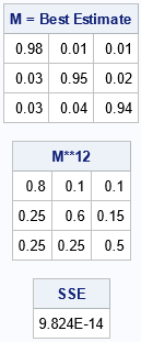
The program shows the estimate for the monthly transition matrix, M, which is the 12th root of the annual transition matrix, T. For this choice of T, there is an exact 12th root. The matrix M¹² is not merely close to T, but it equals T to numeric precision.

A transition matrix that does not have root

In the previous section, the program found a matrix that was exactly the 12th root of the annual transition matrix. This is not always possible. For example, change the target matrix to the following:

/* define the target matrix, T. We want to find the transition matrix, M,
   such that M**12 is as close as possible to the target matrix. */
Target = {0.1 0.4 0.5,
          0.6 0.4   0,
          0     0   1};   * no 12th root for this matrix;

For the people in this survey, everyone who was unemployed last year is still unemployed this year. Furthermore, no one who was employed part-time last year is currently unemployed. Therefore, the transition matrix contains several cells that are zero. It turns out that this matrix does not have a 12th root that is itself a transition matrix. If you rerun the PROC IML program for this annual transition matrix, you get an estimate for the monthly transition matrix, but when you multiply the monthly matrix by itself 12 times, you do not get the original annual matrix. The results are shown below:

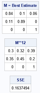
Although this matrix has a small sum of squares of differences (SSE=0.16), the 12th power is not very close to the annual matrix in terms of probabilities. Some of the cells differ by 0.2 or 0.25. Although you have found an estimate for a monthly transition matrix, it isn't a good estimate. Situations like this can occur when the monthly transition matrix is not constant over the 12-month period. For example, hiring in retail and agriculture exhibits seasonal variation.

Using PROC OPTMODEL to solve for a pth root

It is worth mentioning, that the matrix-root problem can have multiple valid solutions. This is not unusual. For example, both +2 and -2 are square roots of the 1 x 1 matrix 4. The 2 x 2 identity matrix has infinitely many square roots because every rotation matrix of the following form is a square root:

R(t) = [ sin(t)   cos(t) ]
       [ cos(t)  -sin(t) ]

Thus, the solution given by the nonlinear optimization algorithm might depend on the initial guess that you provide.

Rob Pratt wrote the following program, which shows how to use PROC OPTMODEL in SAS/OR software to solve the same problem. The program uses the MULTISTART option on the SOLVE statement to specify that the algorithm (an active-set method) will run multiple times, each time using a different initial guess from among a set of uniformly distributed points in the feasible region.

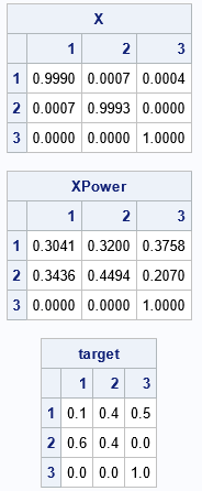
/* The PROC OPTMODEL code was written by Rob Pratt */
proc optmodel;
   set ROWS = 1..3;
   set COLS = ROWS;
   num target {ROWS, COLS} = 
      [0.1 0.4 0.5,
       0.6 0.4   0,
       0     0   1];
   num numPeriods = 12;
   set PERIODS = 1..numPeriods;
 
   var X {i in ROWS, j in COLS} >= 0 <= 1;
   impvar XPower {i in ROWS, j in COLS, p in PERIODS} = 
      (if p = 1 then X[i,j] else sum {k in COLS} XPower[i,k,p-1] * XPower[k,j,p-1]);
   min SSE = sum {i in ROWS, j in COLS} (XPower[i,j,numPeriods] - target[i,j])^2;
   con RowSum {i in ROWS}:
      sum {j in COLS} X[i,j] = 1;
 
   solve with nlp / multistart algorithm=ActiveSet SEED=1234;
   print X 6.4;
   print {i in ROWS, j in COLS} XPower[i,j,numPeriods] 6.4;
   print target;
quit;

The log displays several notes, including the following:

NOTE: 91 distinct local optima were found.
NOTE: The best objective value found by local solver = 0.1745366339.
NOTE: The solution found by local solver with objective = 0.1745366339 was returned.

The notes tell you that the algorithm found 91 distinct local minima. The best solution has an SSE of 0.1745, which is slightly worse than the solution found by using the identity matrix as the initial guess for Newton's method. The procedure displays the following output, which shows that the best solution is close to the identity matrix. This estimate is a valid transition matrix, and the 12th power is close to the target matrix, but is a quite different solution than was found by using PROC IML.

Summary

In summary, this article shows how to use SAS to estimate the root of a Markov transition matrix. This problem is important when you have data that enable you to estimate a transition matrix, T, over a long time period (such as a year), but you want an estimate for a transition matrix, M, over a shorter time period (such as a month) such that M^p = T for a known value of p. In general, this problem does not have an exact solution, but you can find a transition matrix whose pth power is close to the target matrix in a least squares sense. Unfortunately, the root of a matrix is not unique. For some target matrices, you can find many matrices whose pth power is close to the target matrix. This might indicate that the transition matrix is not constant over the shorter time periods.

References

Nicholas J. Higham and Lijing Lin, 2011, "On pth roots of stochastic matrices," Linear Algebra and its Applications, 435 (3), p 448-463.

Blogs