The area under a piecewise linear curve

Recently, I needed to know "how much" of a piecewise linear curve is below the X axis. The coordinates of the curve were given as a set of ordered pairs (x1,y1), (x2,y2), ..., (xn, yn). The question is vague, so the first step is to define the question better. Should I count the number of points on the curve for which the Y value is negative? Should I use a weighted sum and add up all the negative Y values? Ultimately, I decided that the best measure of "negativeness" for my application is to compute the area that lies below the line Y=0 and above the curve. In calculus, this would be the "negative area" of the curve. Because the curve is piecewise linear, you can compute the area exactly by using the trapezoid rule of integration.

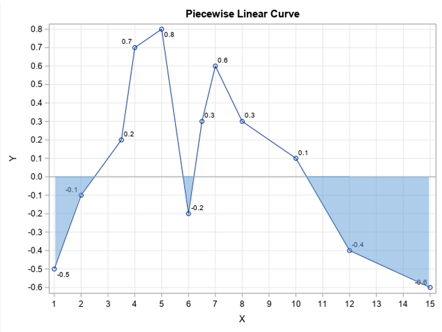
An example is shown to the right. The curve is defined by 12 ordered pairs. The goal of this article is to compute the area shaded in blue. This is the "negative area" with respect to the line Y=0. With very little additional effort, you can generalize the computation to find the area below any horizontal line and above the curve.

Area defined by linear segments

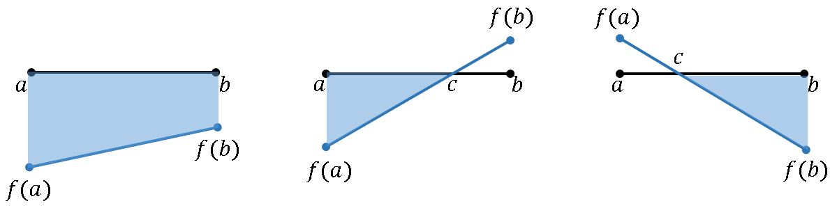
The algorithm for computing the shaded area is simple. For each line segment along the curve, let [a,b] be the interval defined by the left and right abscissas (X values). Let f(a) and f(b) be the corresponding ordinate values. Then there are four possible cases for the positions of f(a) and f(b) relative to the horizontal reference line, Y=0:

Both f(a) and f(b) are above the reference line. In this case, the area between the line segment and the reference line is positive. We are not interested in this case for this article.
Both f(a) and f(b) are below the reference line. In this case, the "negative area" can be computed as the area of a trapezoid: $A = 0.5 (b - a) (f(b) + f(a))$ .
The value f(a) is below the reference line, but f(b) is above the line. In this case, the "negative area" can be computed as the area of a triangle. You first solve for the location, c, at which the line segment intersects the reference line. The negative area is then $A = 0.5 (c - a) f(a)$ .
The value f(a) is above the reference line and f(b) is below the line. Again, the relevant area is a triangle. Solve for the intersection location, c, and compute the negative area as $A = 0.5 (b - c) f(b)$ .

The three cases for negative area are shown in the next figure:

You can easily generalize these formulas if you want the above the curve and below the line Y=t. In every formula that includes f(a), replace that value with (f(a) – t). Similarly, replace f(b) with (f(b) – t).

Compute the negative area

The simplest computation for the negative area is to loop over all n points on the line. For the i_th point (1 ≤ i < n), let [a,b] be the interval [x[i], x[i+1]] and apply the formulas in the previous section. Since we skip any intervals for which f(a) and f(b) are both positive, we can exclude the point (x[i], y[i]) if y[i-1], y[i], and y[i+1] are all positive. This is implemented in the following SAS/IML function. By default, the function returns the area below the line Y=0 and the curve. You can use an optional argument to change the value of the horizontal reference line.

proc iml;
/* compute the area below the line y=y0 for a piecewise
   linear function with vertices given by (x[i],y[i]) */
start AreaBelow(x, y, y0=0);
   n = nrow(x);
   idx = loc(y<y0);                /* find indices for which y[i] < 0 */
   if ncol(idx)=0 then return(0);
 
   k = unique(idx-1, idx, idx+1);  /* we need indices before and after */
   jdx = loc(k > 0 & k <  n);      /* restrict to indices in [1, n-1] */
   v = k[jdx];                     /* a vector of the relevant vertices */
 
   NegArea = 0;
   do j = 1 to nrow(v);            /* loop over intervals where f(a) or f(b) negative */
      i = v[j];                    /* get j_th index in the vector v */
      fa = y[i]-y0; fb = y[i+1]-y0;/* signed distance from cutoff line */
      if fa > 0 & fb > 0 then 
         ;                         /* segment is above cutoff; do nothing */
      else do;
         a  = x[i];  b = x[i+1];
         if fa < 0 & fb < 0 then do;  /* same sign, use trapezoid rule */
            Area = 0.5*(b - a) * (fb + fa);
         end;
         /* different sign, f(a) < 0, find root and use triangle area */
         else if fa < 0 then do;  
            c = a - fa * (b - a) / (fb - fa);
            Area = 0.5*(c - a)*fa;
         end;
         /* different sign, f(b) < 0, find root and use triangle area */
         else do;
            c = a - fa * (b - a) / (fb - fa);
            Area = 0.5*(b - c)*fb;
         end;
         NegArea = NegArea + Area;
      end;
   end;
   return( NegArea );
finish;
 
/* points along a piecewise linear curve */
x = {   1,    2, 3.5,   4,5,     6, 6.5,   7,   8,  10, 12,  15};
y = {-0.5, -0.1, 0.2, 0.7,0.8,-0.2, 0.3, 0.6, 0.3, 0.1,-0.4,-0.6};
 
/* compute area under the line Y=0 and above curve (="negative area") */
NegArea = AreaBelow(x,y);
print NegArea;

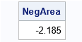
The program defines the AreaBelow function and calls the function for the piecewise linear curve that is shown at the top of this article. The output shows that the area of the shaded regions is -2.185.

The area between a curve and a reference line

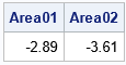
I wrote the program in the previous section so that the default behavior is to compute the area below the reference line Y=0 and above a curve. However, you can use the third argument to specify the value of the reference line. For example, the following statements compute the areas below the lines Y=0.1 and Y=0.2, respectively:

Area01 = AreaBelow(x,y, 0.1);      /* reference line Y=0.1 */
Area02 = AreaBelow(x,y, 0.2);      /* reference line Y=0.2 */
print Area01 Area02;

As you would expect, the magnitude of the area increases as the reference line moves up. In fact, you can visualize the area below the line Y=t and the curve as a function of t. Simply, call the AreaBelow function in a loop for a sequence of increasing t values and plot the results:

t = do(-0.7, 1.0, 0.05);
AreaUnder = j(1,ncol(t));
do i = 1 to ncol(t);
   AreaUnder[i] = AreaBelow(x, y, t[i]);
end;
title "Area Under Reference Line";
call series(t, AreaUnder) label={'Reference Level' 'Area'} grid={x y} xvalues=do(-0.7, 1.0, 0.1);

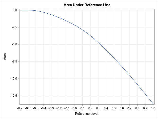
The graph shows that the area under the reference line is a monotonic function. If the reference line is below the minimum value of the curve, the area is zero. As you increase t, the area below the line Y=t and the curve increases in magnitude. After the reference line reaches the maximum value along the curve (Y=0.8 for this example), the magnitude of the area increases linearly. It is difficult to see in the graph above, but the curve is actually linear for t ≥ 0.8.

Summary

You can use numerical integration to determine "how much" of a function is negative. If the function is piecewise linear, the integral over the negative intervals can be computed by using the trapezoid rule. This article shows how to compute the area between a reference line Y=t and a piecewise linear curve. When t=0, this is the "negative area" of the curve.

Incidentally, this article is motivated by the same project that inspired me to write about how to test whether a function is monotonically increasing. If a function is monotonically increasing, then its derivative is strictly positive. Therefore, another way to test a function for monotonic increasing is to test whether the derivative is never negative. A way to measure how far a function deviates from being monotonic is to compute the "negative area" for the derivative.

Blogs