A SAS customer asked how to use the Box-Cox transformation to normalize a single variable. Recall that a normalizing transformation is a function that attempts to convert a set of data to be as nearly normal as possible. For positive-valued data, introductory statistics courses often mention the log transformation or the square-root transformation as possible ways to eliminate skewness and normalize the data. Both of these transformations are part of the family of power transformations that are known as the Box-Cox transformations. A previous article provides the formulas for the Box-Cox transformation.

Formally, a Box-Cox transformation is a transformation of the dependent variable in a regression model. However, the documentation of the TRANSREG procedure contains an example that shows how to perform a one-variable transformation. The trick is to formulate the problem as an intercept-only regression model. This article shows how to perform a univariate Box-Cox transformation in SAS.

A normalizing transformation

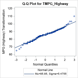
Let's look at the distribution of some data and then try to transform it to become "more normal." The following call to PROC UNIVARIATE creates a histogram and normal quantile-quantile (Q-Q) plot for the MPG_Highway variable in the Sashelp.Cars data set:

%let dsName = Sashelp.Cars;    /* name of data set */
%let YName = MPG_Highway;      /* name of variable to transform */
 
proc univariate data=&dsName;
   histogram &YName / normal;
   qqplot &YName / normal(mu=est sigma=est);
   ods select histogram qqplot;
run;

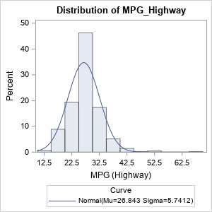
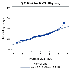
The histogram shows that the data are skewed to the right. This is also seen in the Q-Q plot, which shows a point pattern that is concave up.

You can use a Box-Cox transformation to attempt to normalize the distribution of the data. But you must formulate the problem as an intercept-only regression model. To use the TRANSREG procedure for the Box-Cox transformation, do the following:

• The syntax for PROC TRANSREG requires an independent variable (regressor). To perform an intercept-only regression, you need to manufacture a constant variable and specify it on the right-hand side of the MODEL statement.
• The procedure will complain that the independent variable is constant, but you can add the NOZEROCONSTANT option to suppress the warning.
• Optionally, the documentation for PROC TRANSREG points out that you can improve efficiency by using the MAXITER=0 option.

Notice that the values of the response variable are all positive, therefore we can perform a Box-Cox transformation without having to shift the data. The following statements use a DATA step view to create a new constant variable named _ZERO. The call to PROC TRANSREG uses an intercept-only regression model to transform the response variable:

data AddZero / view=AddZero;
   set &dsName;
   _zero = 0;     /* add a constant variable to use for an intercept-only model */
run;
 
proc transreg data=AddZero details maxiter=0 nozeroconstant;
   model BoxCox(&YName / geometricmean convenient lambda=-2 to 2 by 0.05) = identity(_zero);
   output out=TransOut;    /* write transformed variable to data set */
run;

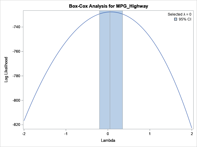
The graph is fully explained in my previous article about the Box-Cox transformation. In the graph, the horizontal axis represents the value of the λ parameter in the Box-Cox transformation. For this example, the LAMBDA= option in the BOXCOX transformation specifies values for λ in the interval [-2, 2]. The vertical axis shows the value of the normal log-likelihood function for the residuals after the dependent variable is transformed for each value of λ. The maximum value of the parameter occurs when λ=0.05. However, because the CONVENIENT option was used and because λ=0 is included in the confidence interval for the optimal value (and is "convenient"), the procedure selects λ=0 for the transformation. The Box-Cox transformation for λ=0 is the logarithmic transformation Y → G*log(Y) where G is the geometric mean of the response variable. (If you do not want to scale by using the geometric mean, omit the GEOMETRICMEAN option in the BOXCOX transformation.)

To summarize, the Box-Cox method selects a logarithmic transformation as the power transformation that makes the residuals "most normal." In an intercept-only regression, the distribution of the residuals is the same as the distribution of the centered data. Consequently, this process results in a transformation that makes the response variable as normally distributed as possible, within the family of power transformations.

Visualize the transformed variable

You can use PROC UNIVARIATE to visualize the distribution of the transformed variable, as follows:

proc univariate data=TransOut;
   histogram T&YName / normal kernel;
   qqplot T&YName / normal(mu=est sigma=est);
   ods select histogram qqplot;
run;

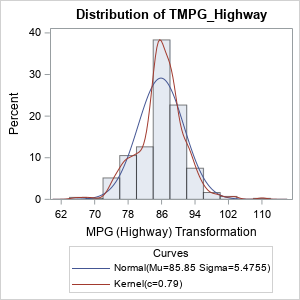
The distribution of the transformed variable is symmetric. The distribution is not perfectly normal (it never will be). In the Q-Q plot, the point pattern shows quantiles that are below the diagonal line on the left and above the line on the right. This indicates outliers (with respect to normality) at both ends of the data distribution.

Summary

This article shows how to perform a Box-Cox transformation of a single variable in SAS. The Box-Cox transformation is intended for regression models, so the trick is to run an intercept-only regression model. To do this, you can use a SAS DATA view to create a constant variable and then use that variable as a regressor in PROC TRANSREG. The procedure produces a Box-Cox plot, which visualizes the normality of the transformed variable for each value of the power-transformation parameter. The parameter value that maximizes the normal log-likelihood function is the best parameter to choose, but in many circumstances, you can use a nearby "convenient" parameter value. The convenient parameter is more interpretable because it favors well-known transformations such as the square-root, logarithmic, and reciprocal transformations.

Appendix: Derivation of logarithm as the limiting Box-Cox transformation

Upon first glance, it is not clear why the logarithm is the correct limiting form of the Box-Cox power transformations as the parameter λ → 0. The power transformations have the form $(x^\lambda - 1)/\lambda$. If you rewrite $x^\lambda = \exp(\lambda \log(x))$ and use the Taylor series expansion of $\exp(z)$ near z=0, you obtain
$\frac{\exp(\lambda \log(x)) - 1}{\lambda} = \frac{(1 + \lambda \log(x) + \lambda^2/2 \log^2(x) + \cdots) - 1}{\lambda} \approx \log(x)$ as λ → 0.