In The Essential Guide to Bootstrapping in SAS, I note that there are many SAS procedures that support bootstrap estimates without requiring the analyst to write a program. I have previously written about using bootstrap options in the TTEST procedure. This article discusses the NLIN procedure, which can fit nonlinear models to data by using a least-squares method. The NLIN procedure supports the BOOTSTRAP statement, which enables you to compute bootstrap estimates of the model parameters. In nonlinear models, the sampling distribution of a regression estimate is often non-normal, so bootstrap confidence intervals can be more useful than the traditional Wald-type confidence intervals that assume the estimates are normally distributed.

Data for a dose-response curve

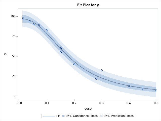
The documentation for PROC NLIN contains an example of fitting a parametric dose-response curve to data. The example only has seven observations, but I have created an additional seven (fake) observations to make the example richer. The graph to the right visualizes the data and a parametric dose-response curve that is fit by using PROC NLIN. The curve represents the expected value of the log-logistic model
$f(x) = \delta + \frac{\alpha - \delta }{1+\gamma \exp \left\{ \beta \ln (x)\right\} }$
where x is the dose. The response is assumed to be bounded in the interval [δ, α], where δ is the response for x=0, and α is the limit of the response as x → ∞. The parameters β and γ determine the shape of the dose-response curve. In the following example, δ=0, and the data suggest that α ≈ 100.

The graph to the right demonstrates the data and the dose-response curve that best fits this data in a least-squares sense.

The following DATA step defines the data. The call to PROC NLIN specifies the model and produces the graph as well as a table of parameter estimates and the correlation between the regression parameters:

data DoseResponse;
   input dose y @@;
   logdose = log(dose);
datalines;
0.009   96.56   0.035   94.12   0.07    89.76
0.15    60.21   0.20    39.95   0.28    21.88
0.50     7.46   0.01    98.1    0.05    90.2
0.10    83.6    0.15    55.1    0.30    32.5
0.40    12.8    0.45     9.6
;
 
proc nlin data=DoseResponse plots(stats=none)=(fitplot); /* request the fit plot */
   parameters alpha=100 beta=3 gamma=300;                /* three parameter model */
   delta = 0;                                            /* a constant; not a parameter */
   Switch = 1/(1+gamma*exp(beta*log(dose)));             /* log-logistic function */
   model y = delta + (alpha - delta)*Switch;
run;

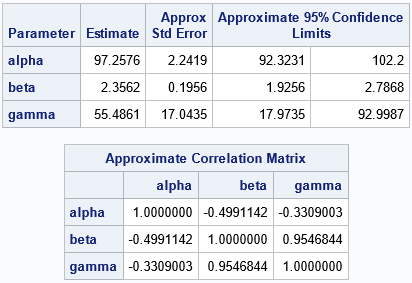
Look at the statistics for the standard errors, the confidence intervals (CIs), and the correlation of the parameters. Notice that these columns contain the word "Approximate" (or "Approx") in the column headers. That is because these statistics are computed by using the formulas from linear regression models. Under the assumptions of ordinary linear regression, the estimates for the regression coefficients are (asymptotically) distributed according to a multivariate normal distribution. For nonlinear regression models, you do not know the sampling distribution of the parameter estimates in advance. However, you can use bootstrap methods to explore the sampling distribution and to improve the estimates of standard error, confidence intervals, and the correlation of the parameters.

The BOOTSTRAP statement in PROC NLIN

You could carry out the bootstrap manually, but PROC NLIN supports the BOOTSTRAP statement, which automatically runs a bootstrap analysis for the regression coefficients. The BOOTSTRAP statement supports the following options:

• Use the SEED= option to specify the random-number stream.
• Use the NSAMPLES= option to specify the number of bootstrap samples that you want to use to make inferences. I suggest at least 1000, and 5000 or 10000 are better values.
• Use the BOOTCI option to request bootstrap confidence intervals for the regression parameters. You can use the BOOTCI(BC) suboption to request the bias-corrected and adjusted method. Use the BOOTCI(PERC) option for the traditional percentile-based confidence intervals. I recommend the bias-corrected option, which is the default.
• Use the BOOTCOV option to display a table that shows the estimated covariance between parameters.
• Use the BOOTPLOTS option to produce histograms of the bootstrap statistics for each regression parameter.

The following call to PROC NLIN repeats the previous analysis, but this time requests a bootstrap analysis to improve the estimates of standard error, CIs, and covariance between parameters:

proc nlin data=DoseResponse plots(stats=none)=(fitplot); /* request the fit plot */
   parameters alpha=100 beta=3 gamma=300;                /* three parameter model */
   delta = 0;                                            /* a constant; not a parameter */
   Switch = 1/(1+gamma*exp(beta*log(dose)));             /* log-logistic function */
   model y = delta + (alpha - delta)*Switch;
   BOOTSTRAP / seed=12345 nsamples=5000 bootci(/*BC*/) bootcov bootplots;
run;
run;

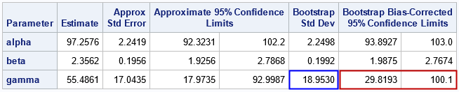
The Parameter Estimates table is the most important output because it shows the bootstrap estimates for the standard error and CIs. For these data, you can see that the estimates for the alpha and beta parameters are not very different from the approximate estimates. However, the estimates for the gamma parameter are quite different. The bootstrap standard error is almost 2 units wider. The bootstrap bias-corrected confidence interval is about 5 units shorter and is shifted to the right as compared to the traditional CI.

You can study the bootstrap distribution of the gamma parameter to understand the differences. The following histogram is produced automatically by PROC NLIN because we used the BOOTPLOTS option. You can see that the distribution of the gamma estimates is not normal. It shows a moderate amount of positive skewness and kurtosis. Thus, the bootstrap estimates are noticeably different from the traditional estimates.

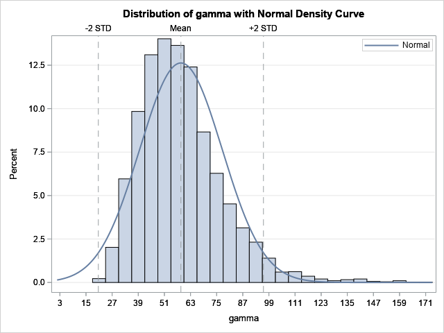
The distributions for the alpha and beta statistics are not shown, but they display only small deviations from normality. Thus, the bootstrap estimates for the alpha and beta parameters are not very different from the traditional estimates.

I do not show the bootstrap estimates of the covariance of the parameters. However, if you convert the bootstrap estimates of covariance to a correlation matrix, you will find that the bootstrap estimates are close to the approximate estimates that are shown earlier.

Summary

The BOOTSTRAP statement in PROC NLIN makes it easy to perform a bootstrap analysis of the regression estimates for a nonlinear regression model. The BOOTSTRAP statement will automatically produce bootstrap estimates of the standard error, confidence intervals, and covariance of parameters. In addition, you can use the BOOTPLOTS option to visualize the bootstrap distribution of the estimates. As shown in this example, sometimes the distribution of a parameter estimate is non-normal, so a bootstrap analysis produces better inferential statistics for the regression analysis.