This article shows how to compute properties of a discrete probability distribution from basic definitions. You can use the definitions to compute the mean, variance, and median of a discrete probability distribution when there is no simple formula for those quantities.

This article is motivated by two computational questions about discrete probability distributions. The first question came from a SAS customer who asked how to calculate the mean of a discrete probability distribution. The second question concerns the median of the binomial distribution, which is an example of a discrete probability distribution. When I was looking up the binomial distribution on Wikipedia, and read the following sentence: "In general, there is no single formula to find the median for a binomial distribution." This led me to think about how software computes the median of discrete distributions.

Moments of a discrete probability distribution

Let X be a discrete random variable with density function f. We assume that X has a well-defined mean, variance, skewness, and kurtosis.

The mean value of X is the first moment of f. The mean is computed as a weighted average of the density values: μ = Σ_i x_i f(x_i),
where the sum is over all possible values of X.

The variance, skewness, and kurtosis of a probability distribution are all central moments. They are also defined as weighted sums where the weights are powers of the deviation from the mean. For example, the variance of any discrete distribution is the second central moment: σ² = Σ_i (x_i – μ)² f(x_i).

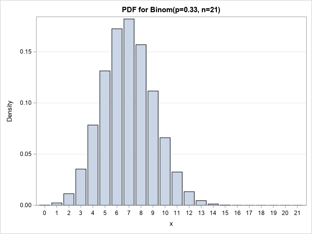
Let's see how to compute the mean and the variance by using SAS. To demonstrate, let's use the binomial distribution with parameters p=0.33 and n=21. That is, X ~ Binom(p, n) gives the number of successes in n=21 independent trials where the probability of success is p=0.33 for each trial. For these parameters, X can take values in the range {0,1,2,...,21}. A graph of the density function is shown to the right;

The mean and variance of the binomial distribution are known to be μ = np and σ² = np(1-p), respectively, so we can check that our computations are correct.

You can use the SAS DATA step to compute these quantities, but I will demonstrate the formulas by using the IML procedure:

proc iml;
p = 0.33;                      /* prob of success for each trial */
n = 21;                        /* number of independent trioals */
 
/* apply the definitions */
x = 0:n;                       /* all possible values of X */
pdf = pdf("Binom", x, p, n);   /* density=pdf(), or use density formula */
meanDef = sum(x#pdf);          /* or inner product x`*pdf */
varDef  = sum((x-meanDef)##2 # pdf);
 
/* Check by using the formulas for Binom(p, n):
   mean = n*p   -and-   variance = n*p*(1-p)
*/
mu = n*p;
var = n*p*(1-p);
print p n meanDef mu varDef var;

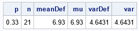
In the program, the mean and variance are computed from first principles by using the definition of the mean and variance. You can perform this computation for any discrete distribution. For the binomial distribution, there are simple formulas for the mean and variance. The output shows that the formulas agree with the computation.

In this example, the range of the discrete random variable is finite, so it is easy to sum over all possible values of X. If X can take on infinitely many values, the computation becomes more complicated. Examples of distributions that have an infinite domain for the density include the geometric distribution and the Poison distribution. For distributions like these, the density must decrease geometrically, so there is some large number N such that for |X|>N the probability in the tails of the distribution is negligible. This reduces the computation to a finite sum.

The definition of the median of a discrete distribution

In many textbooks, the median for a discrete distribution is defined as the value X=m such that at least 50% of the probability is less than or equal to m and at least 50% of the probability is greater than or equal to m. In symbols, P(X≤m) ≤ 1/2 and P(X≥m) ≤ 1/2.

Unfortunately, this definition might not produce a unique median. For example, the binomial distribution Binom(p=0.5, n=21) does not have a unique median because:

• m=10 is a median because P(X≤10) = 0.5 and P(X≥10) ≥ 0.5.
• By symmetry, m=11 is a median because P(X≤11) ≥ 0.5 and P(X≥11) = 0.5.

By convention, most software reports the median to be the LEAST such number that satisfies the definition. So, for the Binom(p=0.5, n=21) distribution, most software reports 10, not 11, as the median.

With this convention, you can compute the median from first principles by summing the densities and reporting the first value of X for which the cumulative density equals or exceeds 0.5. The following statements compute the median for Binom(p=0.33, n=21) by using the definition and check the answer by using the SAS QUANTILE function:

/* use the definition of median to find the first value of X for which CDF >= 0.5 */
cdf = cusum(pdf);
GEHalf = loc(cdf >= 0.5);
medianDef = x[ GEHalf[1] ];  /* first value where CDF >= 1/2 */
 
/* check by calling the built-in QUANTILE function */
median = quantile("Binom", 0.5, p, n); 
print p n medianDef median;

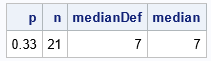
The Wikipedia article states that the median is either FLOOR(n p) or CEIL(n p) and discusses special cases for which the median is ROUND(n p). However, there is no simple formula that works for all cases.

Summary

Although many well-known probability distributions have simple formulas for the mean, variance, and median of the distribution, not all distributions have formulas. This article shows how to compute the mean, variance, and median of a discrete probability distribution from basic definitions. If the random variable X has density function f, then:

• The mean is μ = Σ_i x_i f(x_i)
• The variance is σ² = Σ_i (x_i – μ) ² f(x_i)
• The median, m, is the smallest value of X for which P(X≤m) ≥ 1/2.

The article shows how to compute these quantities in SAS by using SAS/IML software. I leave the DATA step computation for an exercise.