Simulate events when some probabilities are zero

Several probability distributions model the outcomes of various trials when the probabilities of certain events are given. For some distributions, the definitions make sense even when a probability is 0. For other distributions, the definitions do not make sense unless all probabilities are strictly positive. This article examines how zero probabilities affect some common probability distributions, and how to simulate events in SAS when a probability is 0. However, the same techniques can be used to detect and handle other situations where an invalid parameter is used as an argument to a SAS function.

Elementary distributions and event-trial scenarios

The following discrete probability distributions are usually presented in an introductory statistics course. They describe how likely it is to observe one or more events when you run one or more trials. In the following, X is a random variable and p is the probability of success in one Bernoulli trial.

X follows the Bernoulli(p) distribution if P(X=1) = p and P(X=0) = 1 - p.
X follows the Binomial(p, k) distribution if it is the sum of k independent Bernoulli random variable.
X follows a Table(p₁, p₂, ..., p_d) distribution if P(X=X_i) = p_i is the probability that X takes on the i_th value in a set of d values, where the probability of observing the i_th value is p_i.
X follows a Geometric(p) distribution if X is the number of failures until the first success in a sequence of independent Bernoulli trials, each with probability of success p.
X follows a NegativeBinomial(p, k) distribution if X is the number of failures before k successes in a sequence of independent Bernoulli trials, each with probability of success p.

Among these distributions, the Bernoulli and binomial distributions make sense if p=0. In that case, the random variable always has the value 0 because no successes are ever observed. The Table distribution can handle p_i=0, but it usually is advisable to remove the categories that have zero probabilities. However, the geometric and negative binomial distributions are not well-defined if p=0.

Simulation in the SAS DATA step

What happens if you use p=0 for these five distributions? The result might depend on the software you use. The following SAS DATA shows what happens in SAS:

%let NSim = 200;         /* sample size */
data Sample; 
/* define array so that sum(prob)=1 */
array prob[10] _temporary_ (0 0.2 0.125 0.2 0 0.25 0 0.125 0 0.1); 
call streaminit(54321); 
p = 0;                   /* p=0 might cause errors */
k = 10;
do i = 1 to &NSim;
   /* For some distributions, p=0 is okay. */
   /* Success (1) or failure (0) of one trial when Prob(success)=p. */
   Bern = rand("Bernoulli", p);
   /* The number of successes in k indep trials when Prob(success)=p. */
   Bin = rand("Binomial", p, 10);
 
   /* For some distributions, p=0 is questionable, but supported. */
   /* The Table distribution returns a number between 1 and dim(pro)
      when the probability of observing the i_th category is prob[i]. */
   T = rand("Table", of prob[*]);
 
   /* For some distributions, p=0 does not make sense. */
   /* The number of trials that are needed to obtain one success when Prob(success)=p. */
   Geo = rand("Geometric", p);      /* ERROR */
   /* The number of failures before k successes when Prob(success)=p. */
   NB = rand("NegBinomial", p, k);  /* ERROR */
   output; 
end; 
run;

When you run this program, the log will display many notes like the following:

NOTE: Argument 2 to function RAND('Geometric',0) at line 1735
      column 10 is invalid.
NOTE: Argument 2 to function RAND('NegBinomial',0,10) at line
      1737 column 9 is invalid.
<many more notes>
NOTE: Mathematical operations could not be performed at the
      following places. The results of the operations have been
      set to missing values.
<more notes>

The log is telling you that the RAND function considers p=0 to be an invalid argument for the geometric and negative binomial distributions? Why? A geometric random variable shows the number of trials that are needed to obtain one success. But if the probability of success is exactly zero, then we will never observe a success. The number of trials will be infinite. Similarly, a negative binomial random variable shows the number of failures before k successes, but there will never be any successes when p=0. Again, the number of trials will be infinite.

Because the geometric and negative binomial distributions are not defined when p=0, SAS probability routines will note the error and return a missing value, as shown by printing the output data:

proc print data=Sample(obs=5); run;

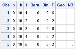
Notice that the Bernoulli and binomial variables are well-defined. Every Bernoulli trial results in X=0, which means that the sum of arbitrarily many trials is also 0. The Table distribution will return only the categories for which the probabilities are nonzero. However, the geometric and negative binomial values are assigned missing values.

Eliminate the notes during a simulation

If you are running a large simulation in which p=0 is a valid possibility, the log will contain many notes. Eventually, SAS will print the following note:

NOTE: Over 100 NOTES, additional NOTES suppressed.

In general, it is a bad idea to suppress notes because there might be additional notes later in the program that you need to see. A better approach is to get rid of all the notes that are telling you that p=0 is an invalid argument. You can do that by using IF-THEN logic to trap the cases where p is very small. For those cases, you can manually assign a missing value. SAS will not issue a note in this case because all calls to SAS functions have valid arguments. This technique is shown in the following DATA step program:

/* workaround: use different logic when p is too small */
%let cutoff = 1e-16;
data Sample2; 
format p Geo NB Best7.;
call streaminit(54321); 
input p @@;
/* The number of trials that are needed to obtain one success when Prob(success)=p. */
if p > &cutoff then 
   Geo = rand("Geometric", p);
else
   Geo = .;
/* The number of failures before k successes when Prob(success)=p. */
if p > &cutoff then 
   NB = rand("NegBinomial", p, 10);  /* k=10 */
else
   NB = .;
datalines;
-0.1  0  1e-20  1e-15 1e-10  1e-6 0.001 0.1
;
 
proc print data=Sample2; run;

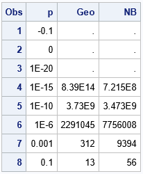
When you run the program, it "runs clean." There are no notes in the log about invalid parameters. The output shows that values of p that are below the cutoff value result in a missing value. Very small values of p that are above the cutoff value are handled by the RAND function, which returns large integers.

Summary

This article discusses how to handle extremely small probabilities in functions that compute probability distributions. The trick is to use IF-THEN logic to prevent the invalid probability from being used as an argument to the RAND function (or other probability functions, such as the PDF, CDF, or QUANTILE functions).

Although this article discusses zero probabilities, this situation is actually a specific case of a larger programming issue: how to prevent notes from appearing in the SAS log when a parameter to a function is invalid. Thus, you can think of this article as yet another example of how to use the "trap and cap" method of defensive programming.

Blogs