Rockin' around the Christmas tree
At the Christmas party hop.
     – Brenda Lee

Last Christmas, I saw a fun blog post that used optimization methods to de-noise an image of a Christmas tree. Although there are specialized algorithms that remove random noise from an image, I am not going to use a specialized de-noising algorithm. Instead, I will use the SVD algorithm, which is a general-purpose matrix algorithm that has many applications. One application is to construct a low-rank approximation of a matrix. This article applies the SVD algorithm to a noisy image of a Christmas tree. The result is recognizable as a Christmas tree, but much of the noise has been eliminated.

A noisy Christmas tree image

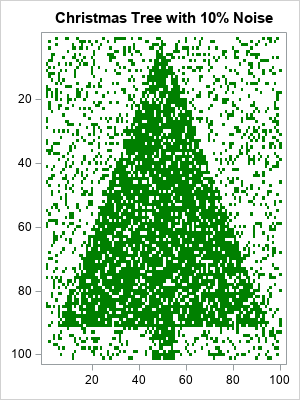
The image to the right is a heat map of a binary (0/1) matrix that has 101 rows and 100 columns. First, I put the value 1 in certain cells so that the heat map resembles a Christmas tree. About 41% of the cells have the value 1. We will call these cells "the tree".

To add random noise to the image, I randomly switched 10% of the cells. The result is an image that is recognizable as a Christmas tree but is very noisy.

Apply the SVD to a matrix

As mentioned earlier, I will attempt to de-noise the matrix (image) by using the general-purpose SVD algorithm, which is available in SAS/IML software. If M is the 101 x 100 binary matrix, then the following SAS/IML statements factor the matrix by using a singular-value decomposition. A series plot displays the first 20 singular values (ordered by magnitude) of the noisy Christmas tree matrix:

call svd(U, D, V, M);                             /* A = U*diag(D)*V` */
call series(1:20, D) grid={x y} xvalues=1:nrow(D) label={"Component" "Singular Value"};

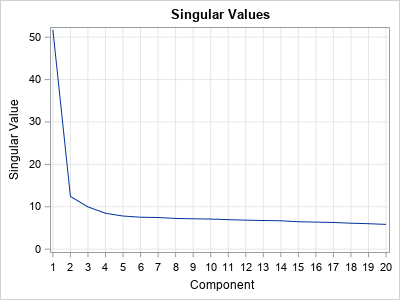
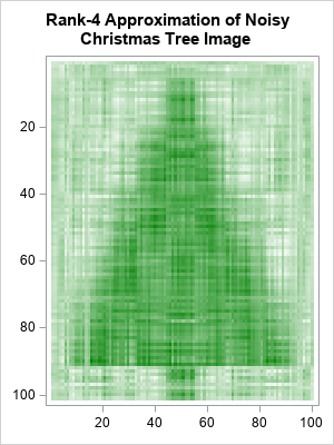
The graph (which is similar to a scree plot in principal component analysis) indicates that the first four singular values are somewhat larger than the remainder. The following statements approximate M by using rank-4 matrix. The rank-4 matrix is not a binary matrix, but you can visualize the rank-4 approximation matrix by using a continuous heat map. For convenience, the matrix elements are shifted and scaled into the interval [0,1].

keep = 4;        /* how many components to keep? */
idx = 1:keep;
Ak = U[ ,idx] * diag(D[idx]) * V[ ,idx]`;
Ak = (Ak - min(Ak)) / range(Ak); /* for plotting, standardize into [0,1] */
s = "Rank " + strip(char(keep)) + " Approximation of Noisy Christmas Tree Image";
call heatmapcont(Ak) colorramp=ramp displayoutlines=0 showlegend=0 title=s range={0, 1};

Apply a threshold cutoff to classify pixels

The continuous heat map shows a dark image of the Christmas tree surrounded by a light-green "fog". The dark-green pixels represent cells that have values near 1. The light-green pixels have smaller values. You can use a histogram to show the distribution of values in the rank-4 matrix:

ods graphics / width=400px height=300px;
call histogram(Ak);

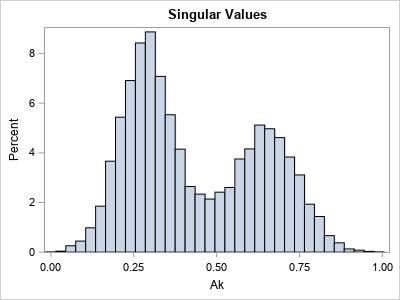
You can think of the cell values as being a "score" that predicts whether each cell belongs to the Christmas tree (green) or not (white). The histogram indicates that the values in the matrix appear to be a mixture of two distributions. The high values in the histogram correspond to dark-green pixels (cells); the low values correspond to light-green pixels. To remove the light-green "fog" in the rank-4 image, you can use a "threshold value" to convert the continuous values to binary (0/1) values. Essentially, this operation predicts which cells are part of the tree and which are not.

For every choice of the threshold parameter, there will be correct and incorrect predictions:

• A "true positive" is a cell that belongs to the tree and is colored green.
• A "false positive" is a cell that does not belong to the tree but is colored green.
• A "true negative" is a cell that does not belong to the tree and is colored white.
• A "false negative" is a cell that belongs to the tree but is colored white.

By looking at the histogram, you might guess that a threshold value of 0.5 will do a good job of separating the low and high values. The following statements use 0.5 to convert the rank-4 matrix into a binary matrix, which you can think of as the predicted values of the de-noising process:

t = 0.5;  /* threshold parameter */
s = "Discrete Filter: Threshold = " + strip(char(t,4,2)) ;
call HeatmapDisc(Ak > t) colorramp=ramp displayoutlines=0 showlegend=0 title=s;

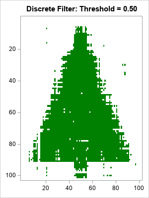
Considering that 10% of the original image was corrupted, the heat map of the reconstructed matrix is impressive. It looks like a Christmas tree, but has much less noise. The reconstructed matrix agrees with the original (pre-noise) matrix for 98% of the cells. In addition:

• There are only a few false positives (green dots) that are far from the tree.
• There are some false negatives in the center of the tree, but many fewer than were in the original noisy image.
• The locations where the image is the most ragged is along the edge and trunk of the Christmas tree. In that region, the de-noising could not tell the difference between tree and non-tree.

The effect of the threshold parameter

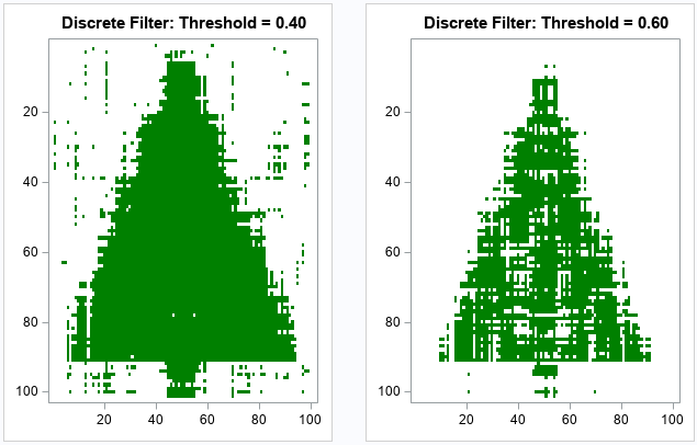
You might wonder what the reconstruction would look like for different choices of the cutoff threshold. The following statements create two other heat maps, one for the threshold value 0.4 and the other for the threshold value 0.6. As you might have guessed, smaller threshold values result in more false positives (green pixels away from the tree), whereas higher threshold values result in more false negatives (white pixels inside the tree).

do t = 0.4 to 0.6 by 0.2;
   s = "Discrete Filter: Threshold = " + strip(char(t,4,2)) ;
   call HeatmapDisc(Ak > t) colorramp=ramp displayoutlines=0 showlegend=0 title=s;
end;

Summary

Although I have presented this experiment in terms of an image of a Christmas tree, it is really a result about matrices and low-rank approximations. I started with a binary 0/1 matrix, and I added noise to 10% of the cells. The SVD factorization enables you to approximate the matrix by using a rank-4 approximation. By using a cutoff threshold, you can approximate the original matrix before the random noise was added. Although the SVD algorithm is a general-purpose algorithm that was not designed for de-noising images, it does a good job eliminating the noise and estimating the original matrix.

If you are interested in exploring these ideas for yourself, you can download the complete SAS program that creates the graphs in this article.