Recently I showed how to visualize and analyze longitudinal data in which subjects are measured at multiple time points. A very common situation is that the data are collected at two time points. For example, in medicine it is very common to measure some quantity (blood pressure, cholesterol, white-blood cell count,...) for each patient before a treatment and then measure the same quantity after an intervention.

This situation leads to pairs of observations. It is useful to visualize the pre/post measurements in a spaghetti plot, a scatter plot, or a histogram of the differences. This article points out that you do not need to create these plots manually: the TTEST procedure can produce all these plots automatically, as well as provide a statistical analysis of paired data.

Visualize pre/post data

When given measurements before and after an intervention (sometimes called "pre/post data"), I like to create a scatter plot of the "before" variable versus the "after" variable. To demonstrate, the following SAS statements define a subset of the data that were analyzed in the previous article. The subset contains 50 children who had high levels of lead in their blood. Lead is toxic, especially in children. The children were given a compound (called succimer) to reduce the blood-lead level and the levels were re-measured one week later.

data PrePost;
   input id lead0 lead1 @@;
   label lead0 = "Baseline Blood Lead Level (mcg/dL)"
         lead1 = "Post-Treatment Blood Lead Level (mcg/dL)";
datalines;
  2   26.5   14.8   3   25.8   23.0  5   20.4    2.8  6   20.4    5.4
 12   24.8   23.1  14   27.9    6.3 19   35.3   25.5 20   28.6   15.8
 22   29.6   15.8  23   21.5    6.5 25   21.8   12.0 26   23.0    4.2
 27   22.2   11.5  29   25.0    3.9 31   26.0   21.4 32   19.7   13.2
 36   29.6   17.5  39   24.4   16.4 40   33.7   14.9 43   26.7    6.4
 44   26.8   20.4  45   20.2   10.6 48   20.2   17.5 49   24.5   10.0
 53   27.1   14.9  54   34.7   39.0 57   24.5    5.1 64   27.7    4.0
 65   24.3   24.3  66   36.6   23.3 68   34.0   10.7 69   32.6   19.0
 70   29.2    9.2  71   26.4   15.3 72   21.8   10.6 79   21.1    5.6
 82   22.1   21.0  85   28.9   12.5 87   19.8   11.6 89   23.5    7.9
 90   29.1   16.8  91   30.3    3.5 93   30.6   28.2 94   22.4    7.1
 95   31.2   10.8  96   31.4    3.9 97   41.1   15.1 98   29.4   22.1
 99   21.9    7.6 100   20.7    8.1
;
 
title "Pre/Post Measurements";
title2 "Created Manually";
proc sgplot data=PrePost aspect=1 noautolegend;
   scatter x=Lead0 y=Lead1 / jitter;
   lineparm x=0 y=0 slope=1 / clip;
   xaxis grid;
   yaxis grid;
run;

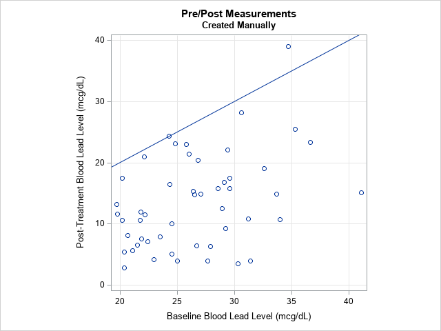
The graph shows the initial measurement (on the X axis) versus the post-treatment measurement (on the Y axis) for each patient in the study. The diagonal line is the identity line. A marker above the line indicates a patient whose measurement increased after treatment. A marker below the line indicates a patient whose measurement decreased. For these data, most children experienced a decrease in blood-lead levels, which indicates that the treatment was effective.

Use PROC TTEST to visualize pre/post data

The goal of ODS statistical graphics in SAS procedures is to provide an analyst with standard visualizations of data that can accompany and enhance a statistical analysis. For pre/post data, a common analysis is to perform a paired t test for the mean difference between the pre- and post-intervention measurements. It turns out that if you run a PROC TTEST analysis, the output not only includes statistical tables but also three common graphs that visualize the data. If the data are in "wide form," the PROC TTEST syntax is simple:

ods graphics on;
proc ttest data=PrePost;
   paired Lead0*Lead1;
run;

Think about this syntax: When you type three PROC TTEST statements, you get a statistical analysis AND three standard visualizations! The graphs appear automatically when you turn on ODS graphics, without requiring any effort on your part.

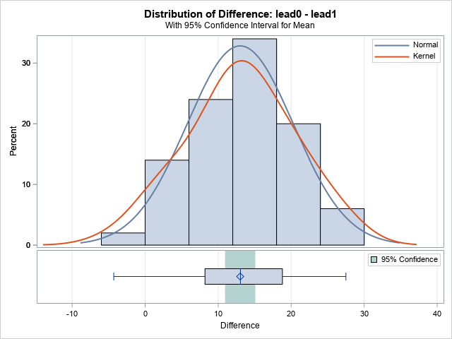
The first graph from PROC TTEST is a histogram of the difference (pre-treatment minus post-treatment). The graph is actually a panel, with a small horizontal box plot underneath that gives another view of the distribution of the differences. You can see that the differences range from -5 to 28. The median change appears to be 13 and the interquartile range is from 8 to 18. If the differences are approximately normally distributed, the light green rectangle indicates a 95% confidence interval for the mean.

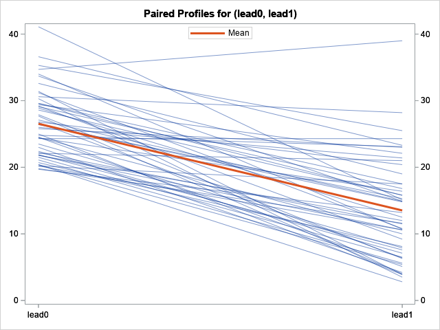
The second graph is a spaghetti plot of the patient profiles. Each line segment represents a patient. The lines connect the pre-treatment values (on the left) to the post-treatment values (on the right). You can see that most (but not all) patients experienced a decrease in blood-lead levels. The red line in the graph indicates the mean pre- and post-treatment levels.

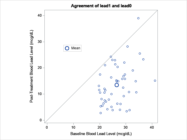
The third graph is a version of the scatter plot that I created earlier by using PROC SGPLOT. Like my version, the graph includes a diagonal reference line. In addition, the graph displays a symbol that shows the pre- and post-treatment mean values of the response variable. The vertical distance between the mean marker and the reference line indicates the average change since the treatment.

PROC TTEST also creates a fourth graph (not shown), which is a normal Q-Q plot of the difference. This graph is useful if you are assessing the normality of the distribution of differences.

Summary

PROC TTEST creates excellent graphs that enable you to visualize pre/post data. With only a few SAS statements, you can produce three common graphs that visualize the change, presumably due to the treatment. Using PROC TTEST is quicker and easier than creating the graphs yourself. Furthermore, one of the graphs (the histogram/box plot panel) is a graph that is not easily created by using PROC SGPLOT. So next time you want to visualize paired data, reach for PROC TTEST.