The eigenvalues of a matrix are not easy to compute. It is remarkable, therefore, that with relatively simple mental arithmetic, you can obtain bounds for the eigenvalues of a matrix of any size. The bounds are provided by using a marvelous mathematical result known as Gershgorin's Disc Theorem. For certain matrices, you can use Gershgorin's theorem to quickly determine that the matrix is nonsingular or positive definite.

The Gershgorin Disc Theorem appears in Golub and van Loan (p. 357, 4th Ed; p. 320, 3rd Ed), where it is called the Gershgorin Circle Theorem. The theorem states that the eigenvalues of any N x N matrix, A, are contained in the union of N discs in the complex plane. The center of the i_th disc is the i_th diagonal element of A. The radius of the i_th disc is the absolute values of the off-diagonal elements in the i_th row. In symbols,
D_i = {z ∈ C | |z - A_{i i}| ≤ r_i }
where r_i = Σ_{i ≠ j} |A_{i j}|. Although the theorem holds for matrices with complex values, this article only uses real-valued matrices.

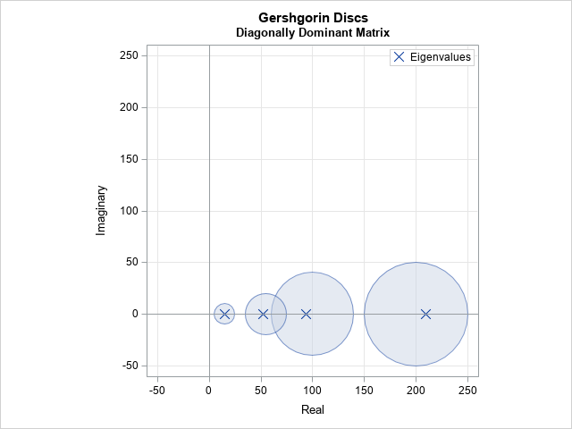
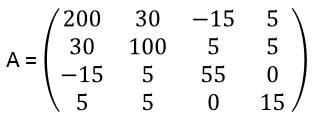
An example of Gershgorin discs is shown to the right. The discs are shown for the following 4 x 4 symmetric matrix:

At first glance, it seems inconceivable that we can know anything about the eigenvalues without actually computing them. However, two mathematical theorems tells us quite a lot about the eigenvalues of this matrix, just by inspection. First, because the matrix is real and symmetric, the Spectral Theorem tells us that all eigenvalues are real. Second, the Gershgorin Disc Theorem says that the four eigenvalues are contained in the union of the following discs:

• The first row produces a disc centered at x = 200. The disc has radius |30| + |-15| + |5| = 50.
• The second row produces a disc centered at x = 100 with radius |30| + |5| + |5| = 40.
• The third row produces a disc centered at x = 55 with radius |-15| + |5| + |0| = 20.
• The last row produces a disc centered at x = 15 with radius |5| + |5| + |0| = 10.

Although the eigenvalues for this matrix are real, the Gershgorin discs are in the complex plane. The discs are visualized in the graph at the top of this article. The true eigenvalues of the matrix are shown inside the discs.

For this example, each disc contains an eigenvalue, but that is not true in general. (For example, the matrix A = {1 −1, 2 −1} does not have any eigenvalues in the disc centered at x=1.) What is true, however, is that disjoint unions of discs must contain as many eigenvalues as the number of discs in each disjoint region. For this matrix, the discs centered at x=15 and x=200 are disjoint. Therefore they each contain an eigenvalue. The union of the other two discs must contain two eigenvalues, but, in general, the eigenvalues can be anywhere in the union of the discs.

The visualization shows that the eigenvalues for this matrix are all positive. That means that the matrix is not only symmetric but also positive definite. You can predict that fact from the Gershgorin discs because no disc intersects the negative X axis.

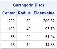
Of course, you don't have to perform the disc calculations in your head. You can write a program that computes the centers and radii of the Gershgorin discs, as shown by the following SAS/IML program, which also computes the eigenvalues for the matrix:

proc iml;
A = { 200  30 -15  5,
       30 100   5  5,
      -15   5  55  0, 
        5   5   0 15};
 
evals = eigval(A);                 /* compute the eigenvalues */
center = vecdiag(A);               /* centers = diagonal elements */
radius = abs(A)[,+] - abs(center); /* sum of abs values of off-diagonal elements of each row */
discs = center || radius || round(evals,0.01);
print discs[c={"Center" "Radius" "Eigenvalue"} L="Gershgorin Discs"];

Diagonally dominant matrices

For this example, the matrix is strictly diagonally dominant. A strictly diagonally dominant matrix is one for which the magnitude of each diagonal element exceeds the sum of the magnitudes of the other elements in the row. In symbols, |A_{i i}| > Σ_{i ≠ j} |A_{i j}| for each i. Geometrically, this means that no Gershgorin disc intersects the origin, which implies that the matrix is nonsingular. So, by inspection, you can determine that his matrix is nonsingular.

Gershgorin discs for correlation matrices

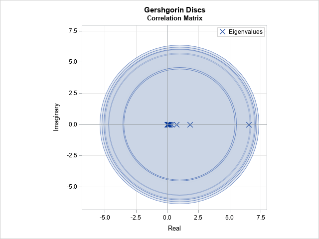
The Gershgorin theorem is most useful when the diagonal elements are distinct. For repeated diagonal elements, it might not tell you much about the location of the eigenvalues. For example, all diagonal elements for a correlation matrix are 1. Consequently, all Gershgorin discs are centered at (1, 0) in the complex plane. The following graph shows the Gershgorin discs and the eigenvalues for a 10 x 10 correlation matrix. The eigenvalues of any 10 x 10 correlation matrix must be real and in the interval [0, 10], so the only new information from the Gershgorin discs is a smaller upper bound on the maximum eigenvalue.

Gershgorin discs for unsymmetric matrices

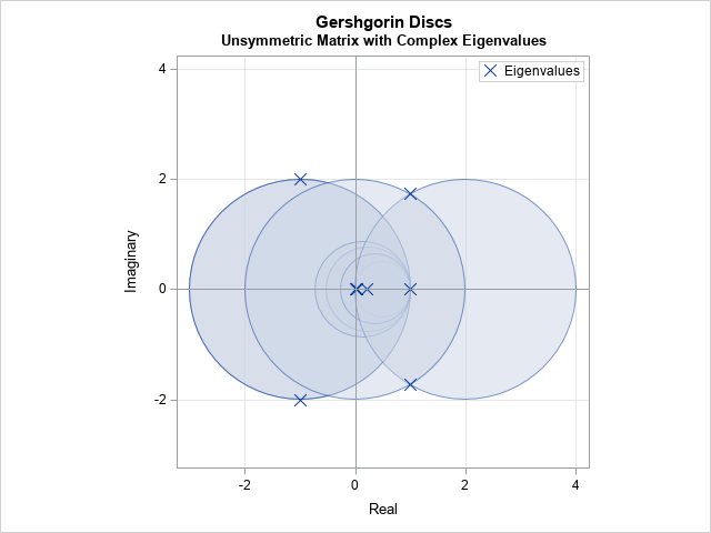
Gershgorin's theorem can be useful for unsymmetric matrices, which can have complex eigenvalues. The SAS/IML documentation contains the following 8 x 8 block-diagonal matrix, which has two pairs of complex eigenvalues:

A = {-1  2  0       0       0       0       0  0,
     -2 -1  0       0       0       0       0  0,
      0  0  0.2379  0.5145  0.1201  0.1275  0  0,
      0  0  0.1943  0.4954  0.1230  0.1873  0  0,
      0  0  0.1827  0.4955  0.1350  0.1868  0  0,
      0  0  0.1084  0.4218  0.1045  0.3653  0  0,
      0  0  0       0       0       0       2  2,
      0  0  0       0       0       0      -2  0 };

The matrix has four smaller Gershgorin discs and three larger discs (radius 2) that are centered at (-1,0), (2,0), and (0,0), respectively. The discs and the actual eigenvalues of this matrix are shown in the following graph. Not only does the Gershgorin theorem bound the magnitude of the real part of the eigenvalues, but it is clear that the imaginary part cannot exceed 2. In fact, this matrix has eigenvalues -1 ± 2 i, which are on the boundary of one of the discs, which shows that the Gershgorin bound is tight.

Conclusions

In summary, the Gershgorin Disc Theorem provides a way to visualize the possible location of eigenvalues in the complex plane. You can use the theorem to provide bounds for the largest and smallest eigenvalues.

I was never taught this theorem in school. I learned it from a talented mathematical friend at SAS. I use this theorem to create examples of matrices that have particular properties, which can be very useful for developing and testing software.

This theorem also helped me to understand the geometry behind "ridging", which is a statistical technique in which positive multiples of the identity are added to a nearly singular X`X matrix. The Gershgorin Disc Theorem shows the effect of ridging a matrix is to translate all of the Gershgorin discs to the right, which moves the eigenvalues away from zero while preserving their relative positions.

You can download the SAS program that I used to create the images in this article.

Further reading

There are several papers on the internet about Gershgorin discs. It is a favorite topic for advanced undergraduate projects in mathematics.

• Brakken-Thal, S. (2007) "Gershgorin’s Theorem for Estimating Eigenvalues"
• Marquis, D. (2016) "Gershgorin’s Circle Theorem for Estimating the Eigenvalues of a Matrix with Known Error Bounds"
• Leinster, T. (2016) "In Praise of the Gershgorin Disc Theorem"