This article describes and implements a fast algorithm that estimates a median for very large samples. The traditional median estimate sorts a sample of size N and returns the middle value (when N is odd). The algorithm in this article uses Monte Carlo techniques to estimate the median much faster.

Of course, there's no such thing as a free lunch. The Monte Carlo estimate is an approximation. It is useful when a quick-and-dirty estimate is more useful than a more precise value that takes longer to compute. For example, if you want to find the median value of 10 billion credit card transactions, it might not matter whether the median $16.74 or $16.75. Either would be an adequate estimate for many business decisions.

Although the traditional sample median is commonly used, it is merely an estimate. All sample quantiles are estimates of a population quantity, and there are many ways to estimate quantiles in statistical software. To estimate these quantities faster, researchers have developed approximate methods such as the piecewise-parabolic algorithm in PROC MEANS or "probabilistic methods" such as the ones in this article.

Example data: A sample from a mixture distribution

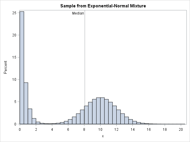
Consider the following data set, which simulates 10 million observations from a mixture of an exponential and a normal distribution. You can compute the exact median for the distribution, which is 8.065. A histogram of the data and the population median are shown to the right.

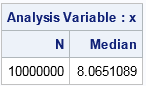
Because the sample size is large, PROC MEANS takes a few seconds to compute the sample median by using the traditional algorithm which sorts the data (an O(N log N) operation) and then returns the middle value. The sample median is 8.065.

/* simulate from a mixture distribution. See
   https://blogs.sas.com/content/iml/2011/09/21/generate-a-random-sample-from-a-mixture-distribution.html */
%let N = 1e7;
data Have;
call streaminit(12345);
do i = 1 to &N;
   d = rand("Bernoulli", 0.6);
   if d = 0 then
      x = rand("Exponential", 0.5);
   else
      x = rand("Normal", 10, 2);
   output;
end;
keep x;
run;
 
/* quantile estimate */
proc means data=Have N Median;
   var x;
run;

A naive resampling algorithm

The basic idea of resampling methods is to extract a random subset of the data and compute statistics on the subset. Although the inferential statistics (standard errors and confidence interval) on the subset are not valid for the original data, the point estimates are typically close, especially when the original data and the subsample are large.

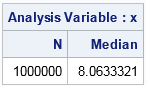
The simplest form of a resampling algorithm is to generate a random subsample of the data and compute the median of the subsample. The following example uses PROC SURVEYSELECT to resample (with replacement) from the data. The subsample is one tenth as large as the original sample. The subsequent call to PROC MEANS computes the median of the subsample, which is 8.063.

proc surveyselect data=Have seed=1234567 NOPRINT 
     out=SubSample
     method=urs samprate=0.1;                 /* 10% sampling with replacement */
run;
 
title "Estimate from 10% of the data";
proc means data=SubSample N Median;
   freq NumberHits;
   var x;
run;

It takes less time to extract a 10% subset and compute the median than it takes to compute the median of the full data. This naive resampling is simple to implement and often works well, as in this case. The estimate on the resampled data is close to the true population median, which is 8.065. (However, the standard error of the traditional estimate is smaller.)

You might worry, however, that by discarding 90% of the data you might discard too much information. In fact, there is a 90% chance that we discarded the middle data value! Thus it is wise to construct the subsample more carefully. The next section constructs a subsample that excludes data from the tails of the distribution and keeps data from the middle of the distribution.

A probabilistic algorithm for the median

This section presents a more sophisticated approximate algorithm for the median. My presentation of this Monte Carlo algorithm is based on the lecture notes of Prof. H-K Hon and a Web page for computer scientists. Unfortunately, neither source credits the original author of this algorithm. If you know the original reference, please post it in the comments.

Begin with a set S that contains N observations. The following algorithm returns an approximate median with high probability:

1. Choose a random sample (with replacement) of size k = N^3/4 from the data. Call the sample R.
2. Choose lower and upper "sentinels," L and U. The sentinels are the lower and upper quantiles of R that correspond to the ranks k/2 ± sqrt(N). These sentinels define a symmetric interval about the median of R.
3. (Optional) Verify that the interval [L, U] contains the median value of the original data.
4. Let C be the subset of the original observations that are within the interval [L, U]. This is a small subset.
5. Return the median of C.

The idea is to use the random sample only to find an interval that probably contains the median. The width of the interval depends on the size of the data. If N=10,000, the algorithm uses the 40th and 60th percentiles of the random subset R. For N=1E8, it uses the 49th and 51th percentiles.

The following SAS/IML program implements the Monte Carlo estimate for the median:

proc iml;
/* Choose a set R of k = N##(3/4) elements in x, chosen  at random with replacement. 
   Choose quantiles of R to form an interval [L,U].
   Return the median of data that are within [L,U]. */
start MedianRand(x);
   N = nrow(x);
   k = ceil(N##0.75);    /* smaller sample size */
   R = T(sample(x, k));  /* bootstrap sample of size k (with replacement) */
   call sort(R);         /* Sort this subset of data */
   L = R[ floor(k/2 - sqrt(N)) ]; /* lower sentinel */
   U = R[  ceil(k/2 + sqrt(N)) ]; /* upper sentinel */
   UTail = (x > L);       /* indicator for large values */
   LTail = (x < U);       /* indicator for small values */
   if sum(UTail) > N/2 & sum(LTail) > N/2 then do;
      C = x[loc(UTail & LTail)]; /* extract central portion of data */
      return ( median(C) );      
   end;
   else do;
      print "Median not between sentinels!";
      return (.);
   end;
finish;
 
/* run the algorithm on example data */
use Have; read all var {"x"}; close;
call randseed(456);
 
t1 = time();
   approxMed = MedianRand(x);  /* compute approximate median; time it */
tApproxMed = time()-t1;
 
t0 = time();
   med = median(x);            /* compute traditional estimate; time it */
tMedian = time()-t0;
 
results = (approxMed || med) // (tApproxMed|| tMedian);
print results[colname={"Approx" "Traditional"}
              rowname={"Estimate" "Time"} F=Best6.];

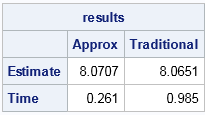
The output indicates that the Monte Carlo algorithm gives an estimate that is close to the traditional estimate, but produces it three times faster. If you repeat this experiment for 1E8 observations, the Monte Carlo algorithm computes an estimate in 2.4 seconds versus 11.4 seconds for the traditional estimate, which is almost five times faster. As the data size grows, the speed advantage of the Monte Carlo algorithm increases. See Prof. Hon's notes for more details.

In summary, this article shows how to implement a probabilistic algorithm for estimating the median for large data. The Monte Carlo algorithm uses a bootstrap subsample to estimate a symmetric interval that probably contains the true median, then uses the interval to strategically choose and analyze only part of the original data. For large data, this Monte Carlo estimate is much faster than the traditional estimate.