For a time series { y₁, y₂, ..., y_N }, the difference operator computes the difference between two observations. The kth-order difference is the series { y_k+1 - y₁, ..., y_N - y_N-k }. In SAS, the DIF function in the DATA step computes differences between observations. The DIF function in the SAS/IML language takes a column vector of values and returns a vector of differences.

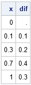
For example, the following SAS/IML statements define a column vector that has five observations and calls the DIF function to compute the first-order differences between adjacent observations. By convention, the DIF function returns a vector that is the same size as the input vector and inserts a missing value in the first element.

proc iml;
x = {0, 0.1, 0.3, 0.7, 1};
dif = dif(x);            /* by default DIF(x, 1) ==> first-order differences */
print x dif;

The difference operator is a linear operator that can be represented by a matrix. The first nonmissing value of the difference is x[2]-x[1], followed by x[3]-x[2], and so forth. Thus the linear operator can be represented by the matrix that has -1 on the main diagonal and +1 on the super-diagonal (above the diagonal). An efficient way to construct the difference operator is to start with the zero matrix and insert ±1 on the diagonal and super-diagonal elements. You can use the DO function to construct the indices for the diagonal and super-diagonal elements in a matrix:

start DifOp(dim);
   D = j(dim-1, dim, 0);        /* allocate zero martrix */
   n = nrow(D); m = ncol(D);
   diagIdx = do(1,n*m, m+1);    /* index diagonal elements */
   superIdx  = do(2,n*m, m+1);  /* index superdiagonal elements */
   *subIdx  = do(m+1,n*m, m+1); /* index subdiagonal elements (optional) */
   D[diagIdx] = -1;             /* assign -1 to diagonal elements */
   D[superIdx] = 1;             /* assign +1 to super-diagonal elements */
   return D;
finish;
 
B = DifOp(nrow(x));
d = B*x;
print B, d[L="Difference"];

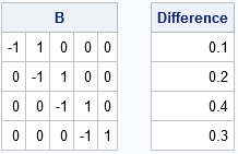
You can see that the DifOp function constructs an (n-1) x n matrix, which is the correct dimension for transforming an n-dimensional vector into an (n-1)-dimensional vector. Notice that the matrix multiplication omits the element that previously held a missing value.

You probably would not use a matrix multiplication in place of the DIF function if you needed the first-order difference for a single time series. However, the matrix formulation makes it possible to use one matrix multiplication to find the difference for many time series.

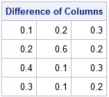
The following matrix contains three time-series, one in each column. The B matrix computes the first-order difference for all columns by using a single matrix-matrix multiplication. The same SAS/IML code is valid whether the X matrix has three columns or three million columns.

/* The matrix can operate on a matrix where each column is a time series */
x = {0    0    0,
     0.1  0.2  0.3,
     0.3  0.8  0.5,
     0.7  0.9  0.8,
     1    1    1   };
B = DifOp(nrow(x));
d = B*x;                        /* apply the difference operator */
print d[L="Difference of Columns"];

Other operators in time series analysis can also be represented by matrices. For example, the first-order lag operator is represented by a matrix that has +1 on the super-diagonal. Moving average operators also have matrix representations.

The matrix formulation is efficient for short time series but is not efficient for a time series that contains thousands of elements. If the time series contains n elements, then the dense-matrix representation of the difference operator contains about n2 elements, which consumes a lot of RAM when n is large. However, as we have seen, the matrix representation of an operator is advantageous when you want to operate on a large number of short time series, as might arise in a simulation.