In some applications, you need to optimize a linear objective function of many variables, subject to linear constraints. Solving this problem is called linear programming or linear optimization. This article shows two ways to solve linear programming problems in SAS: You can use the OPTMODEL procedure in SAS/OR software or use the LPSOLVE function in SAS/IML software.

Formulating the optimization

A linear programming problem can always be written in a standard vector form. In the standard form, the unknown variables are nonnegative, which is written in vector form as x ≥ 0. Because the objective function is linear, it can be expressed as the inner product of a known vector of coefficients (c) with the unknown variable vector: c^Tx Because the constraints are also linear, the inequality constraints can always be written as Ax ≤ b for a known constraint matrix A and a known vector of values b.

In practice, it is often convenient to be able to specify the problem in a non-standardized form in which some of the constraints represent "greater than," others represent "less than," and others represent equality. Computer software can translate the problem into a standardized form and solve it.

A linear programming problem example

As an example of how to solve a linear programming problem in SAS, let's pose a particular two-variable problem:

• Let x = {x1, x2} be the vector of unknown positive variables.
• Define the objective function to maximize as 3*x1 + 5*x2. In vector form, the objective function is c^Tx where c = {3, 5}.
• Define the linear constraints as follows:
  3*x1 + -2*x2 ≤ 10
  5*x1 + 10*x2 ≤ 56
  4*x1 +  2*x2 ≥  7
  In matrix form, you can define the 3 x 2 matrix of constraint coefficients A = {3  -2, 5  10, 4  2} and the right-hand-side vector b = {10, 56, 7}. There is not a standard way to express a "vector of symbols," but we can invent one. Let LEG = {≤, ≤, ≥} be a vector of symbols. ("LEG" is a mnemonic for "Less than," "Equal to," or "Greater than.") With this notation, the vector of constraints is written as Ax LEG b.

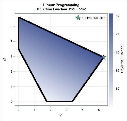
The graph shows the polygonal region in the plane that satisfies the constraints for this problem. The region (called the feasible region) is defined by the two axes and the three linear inequalities. The color in the interior of the region indicates the value of the objective function within the feasible region. The green star indicates the optimal solution, which is x = {5.3, 2.95}.

The theory of linear programming says that an optimal solution will always be found at a vertex of the feasible region, which in 2-D is a polygon. In this problem, the feasible polygon has only five vertices, so you could evaluate the objective function at each vertex by hand to find the optimal solution. For high-dimensional problems, however, you definitely want to use a computer!

Linear programming in SAS by using the OPTMODEL procedure

The OPTMODEL procedure is part of SAS/OR software. It provides a natural programming language with which to define and solve all kinds of optimization problems. The linear programming example in this article is similar to the "Getting Started" example in the PROC OPTMODEL chapter about linear programming. The following statements use syntax that is remarkably similar to the mathematical formulation of the problem:

proc optmodel;
var x{i in 1..2} >= 0;           /* information about the variables */
max z = 3*x[1] +  5*x[2];        /* define the objective function */
con c1: 3*x[1] + -2*x[2] <= 10;  /* specify linear constraints */
con c2: 5*x[1] + 10*x[2] <= 56;
con c3: 4*x[1] +  2*x[2] >=  7;
solve;                           /* solve the LP problem */
print x;

The OPTMODEL procedure prints two tables. The first (not shown) is a table that describes the algorithm that was used to solve the problem. The second table is the solution vector, which is x = {5.3, 2.95}.

For an introduction to using the OPTMODEL procedure to solve linear programming problems, see the 2011 paper by Rob Pratt and Ed Hughes.

Linear programming by using the LPSOLVE subroutine in SAS/IML

Not every SAS customer has a license for SAS/OR software, but hundreds of thousands of people have access to the SAS/IML matrix language. In addition to companies that license SAS/IML software, SAS/IML is part of the free SAS University Edition, which has been downloaded almost one million times by students, teachers, researchers, and self-learners.

Whereas the syntax in PROC OPTMODEL closely reflects the mathematical formulation, the SAS/IML language uses matrices and vectors to specify the problem. You then pass those matrices as arguments to the LPSOLVE subroutine. The subroutine returns the solution (and other information) in output arguments. The following list summarizes the information that you must provide:

• Define the range of the variables: You can specify a vector for the lower bounds and/or upper bounds of the variables.
• Define the objective function: Specify the vector of coefficients (c) such that c`*x is the linear objective function. Specify whether the goal is to minimize or maximize the objective function.
• Specify the linear constraints: Specify the matrix of constraint coefficients (A), the right-hand side vector of values (b), and a vector (LEG) that indicates whether each constraint is an inequality or an equality. (The documentation calls the LEG vector the "rowsense" vector because it specifies the "sense" or direction of each row in the constraint matrix.)

The following SAS/IML program defines and solves the same LP problem as in the previous section. I've added plenty of comments so you can see how the elements in this program compare to the more compact representation in PROC OPTMODEL:

proc iml;
/* information about the variables */
LowerB = {0, 0};           /* lower bound constraints on x */
UpperB = {., .};           /* upper bound constraints on x */
 
/* define the objective function */
c = {3, 5};                /* vector for objective function c*x */
/* control vector for optimization */
ctrl = {-1,                /* maximize objective */
         1};               /* print some details */
 
/* specify linear constraints */
A = {3 -2,                 /* matrix of constraint coefficients */
     5 10,
     4  2};
b = {10,                   /* RHS of constraint eqns (column vector) */
     56,
      7};         
LEG = {L, L, G};           /* specify symbols for constraints:
                              'L' for less than or equal
                              'E' for equal
                              'G' for greater than or equal */
 
/* solve the LP problem */
CALL LPSOLVE(rc, objVal, result, dual, reducost, /* output variables */
             c, A, b,      /* objective and linear constraints */
             ctrl,         /* control vector */
             LEG, /*range*/ , LowerB, UpperB); 
print rc objVal, result[rowname={x1 x2}];

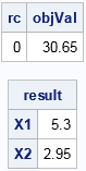
In the call to LPSOLVE, the first five arguments are output arguments. The first three of these are printed:

• If the call finds the optimal solution, then the return code (rc, first parameter) is 0.
• The value of the objective function at the optimal value is returned in the second parameter (objVal).
• The solution to the LP problem (the optimal value of the variables) is returned in the third argument.

Although the LPSOLVE function was not as simple to use as PROC OPTMODEL, it obtains the same solution. The LPSOLVE subroutine supports many features that are not mentioned here. For details, see the documentation for LPSOLVE.

The LPSOLVE subroutine was introduced in SAS/IML 13.1, which was shipped with SAS 9.4m1. The LPSOLVE function replaces the older LP subroutine, which is deprecated. SAS 9.3 customers can call the LP subroutine, which works similarly.