This article shows how to solve mixed integer linear programming (MILP) problems in SAS. In a mixed integer problem, some of the variables in the problem are integer-valued whereas others are continuous. The objective function is a linear function of the variables and the variables can be subject to linear constraints.

Last month I discussed how to solve linear programming (LP) problems in SAS by using PROC OPTMODEL in SAS/OR or by using SAS/IML software. You can use these same tools to solve mixed integer linear programming problems. The OPTMODEL procedure has the simpler syntax. The MILPSOLVE function in SAS/IML software provides similar functionality in an interactive matrix language.

A mixed integer linear programming problem example

The previous article solved a two-variable LP problem. If you constrain one of the variables to be an integer, you get a MILP problem, as follows:

• Let x = {x1, x2} be the vector of unknown positive variables. The x1 variable is integer-valued; the x2 variable is continuous.
• The objective function to maximize is 3*x1 + 5*x2. In vector form, the objective function is c^Tx where c = {3, 5}.
• There are three linear constraints, which you can represent in matrix form. Define the 3 x 2 matrix of constraint coefficients A = {3  -2, 5  10, 4  2} and the right-hand-side vector b = {10, 56, 7}. Let LEG = {≤, ≤, ≥} be a "vector of symbols." ("LEG" is a mnemonic for "Less than," "Equal to," or "Greater than.") With this notation, the vector of constraints is written as Ax LEG b.

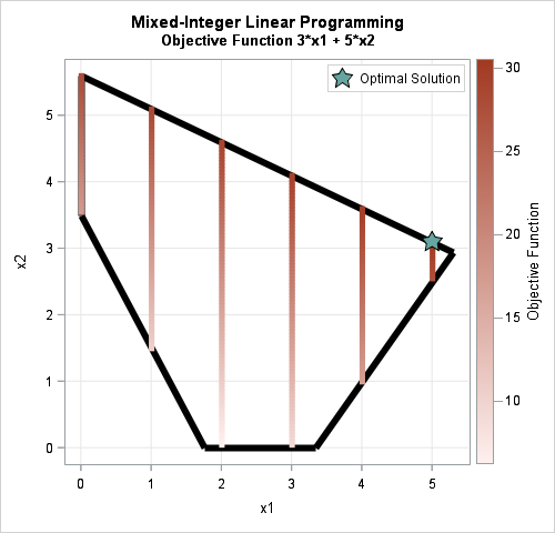
The graph shows the feasible region. The interior of the polygon satisfies the constraints. Because x1 must be an integer, the vertical stripes indicate the feasible values of the variables. The color of the stripes indicate the value of the objective function. The green star indicates the optimal solution, which is x = {5, 3.1}.

Mixed integer linear programming by using the OPTMODEL procedure

The following statements show one way to formulate and solve the MILP problem by using the OPTMODEL procedure in SAS/OR software:

proc optmodel;
var x1 integer >= 0;           /* information about the variables */
var x2 >= 0;
max z = 3*x1 +  5*x2;         /* define the objective function */
con c1: 3*x1 + -2*x2 <= 10;   /* specify linear constraints */
con c2: 5*x1 + 10*x2 <= 56;
con c3: 4*x1 +  2*x2 >=  7;
solve with milp;              /* solve the MILP problem */
print x1 x2;
quit;

The OPTMODEL procedure prints two tables. The first (not shown) describes the optimization algorithm and tells you that the optimal objective value is 30.5. The second table is the solution vector, which is x = {5, 3.1}.

Mixed integer linear programming by using the MILPSOLVE subroutine in SAS/IML

The MILPSOLVE subroutine in the SAS/IML language uses matrices and vectors to specify the problem. The syntax for the MILPSOLVE subroutine is almost identical to the syntax for the LPSOLVE subroutine, so see the previous article for an explanation of each argument. The following SAS/IML program defines and solves the MILP problem:

proc iml;
/* information about variables (row of column, doesn't matter) */
colType = {I, C};  /*  C, B, or I for cont, binary, int */
LowerB =  {0, 0};  /* lower bound constraints on x */
UpperB = {10,10};  /* upper bound constraints on x */
 
/* objective function */
c = {3 5};        /* vector for objective function c*x */
 
/* linear constraints */
A = {3 -2,        /* matrix of constraint coefficients */
     5 10,
     4  2};
b = {10,          /* RHS of constraint eqns (column vector) */
     56,
      7};         
 
/* specify symbols for constraints:
   'L' for less than or equal
   'E' for equal
   'G' for greater than or equal */
LEG = {L, L, G}; 
 
/* control vector for optimization */
ctrl = {-1,       /* maximize objective */
         1};      /* print level */
 
CALL MILPSOLVE(rc, objVal, result, relgap, /* output variables */
               c, A, b,      /* objective and linear constraints */
               ctrl,         /* control vector */
               coltype, LEG, /*range*/, LowerB, UpperB); 
print rc objVal, result[rowname={x1 x2}];

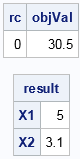
In the call to MILPSOLVE, the first four arguments are output arguments. The return code (rc) is 0, which indicates that an optimal value was found. The value of the objective function at the optimal value is returned in objVal. The optimal values of the variables are returned in the result argument.

The MILPSOLVE subroutine was introduced in SAS/IML 13.1, which was shipped with SAS 9.4m1. For additional details about the MILPSOLVE subroutine, see the documentation.