Last week I blogged about how to draw the Cantor function in SAS. The Cantor function is used in mathematics as a pathological example of a function that is constant almost everywhere yet somehow manages to "climb upwards," thus earning the nickname "the devil's staircase."

The Cantor function has three properties: (1) it is continuous, (2) it is non-decreasing, and (3) F(0)=0 and F(1)=1. There is a theorem that says that any function with these properties is the cumulative distribution function (CDF) for some random variable. In theory, therefore, you can generate a large number of random variates (a large sample), then use PROC UNIVARIATE to plot the empirical CDF. The empirical CDF should be the devil's staircase function.

A random sample from the Cantor set

My last article showed that every point in the Cantor set can be written as the infinite sum x = Σ_i a_i3^-i where the a_i equal 0 or 2. You can approximate the Cantor set by truncating the series at a certain number of terms. You can generate random points from the (approximate) Cantor set by choosing the coefficients randomly from the Bernoulli distribution with probability 0.5. The following DATA step generates 10,000 points from the Cantor set by using random values for the first 20 coefficients:

data Cantor;
call streaminit(123456);
k = 20;             /* maximum number of coefficients */
n = 10000;          /* sample size to generate */
do i = 1 to n;      /* generate n random points in Cantor set */
   x = 0;
   do j = 1 to k;   /* each point is sum of powers of 1/3 */
      b = 2 * rand("Bernoulli", 0.5);  /* random value 0 or 2 */
      x + b * 3**(-j);                 /* power of 1/3 */
   end;
   output;
end;
keep x;
run;
 
proc univariate data=Cantor;
   cdf x;
run;

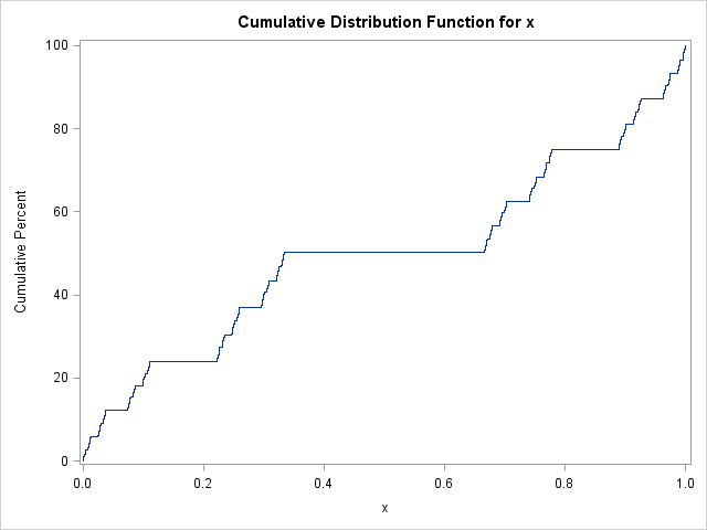
The call to PROC UNIVARIATE displays the empirical CDF for the random sample of points. And voilà! The Cantor distribution function appears! As a bonus, the output from PROC UNIVARIATE (not shown) indicates that the mean of the distribution is 1/2 (which is obvious by symmetry) and the variance is 1/8, which you might not have expected.

This short SAS program does two things: it shows how to simulate a random sample uniformly from the (approximate) Cantor set, and it indicates that the devil's staircase function is the distribution function for this a uniform random variable.

A random sample in SAS/IML

Alternatively, you can generate the same random sample by using SAS/IML and matrix computations. My previous article drew the Cantor function by systematically using all combinations of 0s and 2s to construct the elements of the Cantor set. However, you can use the same matrix-based approach but generate random coefficients, therefore obtaining a random sample from the Cantor set:

proc iml;
k = 20;          /* maximum number of coefficients */
n = 10##4;       /* sample size to generate */
B = 2 * randfun(n||k, "Bernoulli", 0.5);  /* random n x k matrix of 0/2 */
v = 3##(-(1:k)); /* powers of 1/3 */
x = B * v`;      /* sum of random terms that are either 0*power or 2*power */

Recall that ECDF is a step function that plots the ith ordered datum at the height i/n. You can approximate the empirical CDF in SAS/IML by using the SERIES subroutine. Technically, the lines that appear in the line plot have a nonzero slope, but the approximation looks very similar to the PROC UNIVARIATE output:

call sort(x, 1);             /* order elements in the Cantor set */
x = 0 // x // 1;             /* append end points */
y = do(0, 1, 1/(nrow(x)-1)); /* empirical CDF */
title "Empirical Distribution of a Uniform Sample from the Cantor Set";
call series(x, y);

Interpretation in probability

It is interesting that you can actually define the Cantor set in terms of rolling a fair six-sided die. Suppose that you roll a die infinitely often and we adopt the following rules:

• If the die shows a 1 or 2, you get zero points.
• If the die shows a 3 or 4, you get one point.
• If the die shows a 5 or 6, you get two points.

This game is closely related to the Cantor set. Recall that the Cantor set can be written as the set of all base-3 decimal values in [0,1] for which the decimal expansion does not contain a 1. In this game, each point in the Cantor set corresponds to a sequence of rolls that never contain a 3 or 4. (Equivalently, the score is always even.) Obviously this would never happen in real life, which is an intuitive way of saying that the Cantor set has "measure zero."

References

The first time I saw the Cantor function depicted as an empirical distribution function was when I saw a very compact MATLAB formula like this:

x=2*3.^-[1:k]*(rand(k,n)<1/2);
stairs([min(x) sort(x)],0:1/length(x):1) % Plot the c.d.f of x

The previous formula is equivalent to my SAS/IML program, but in my program I broke the formula apart so that the components could be understood more easily. This formula appears in a set of probability demos by Peter Doyle. I had the privilege to interact with Professor Doyle at The Geometry Center (U. MN) in the early 1990s, so perhaps he was responsible for showing me the Cantor distribution.

These UNC course notes from Jan Hannig also discuss the Cantor distribution, but the original source is not cited.