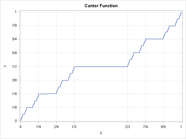
I was a freshman in college the first time I saw the Cantor middle-thirds set and the related Cantor "Devil's staircase" function. (Shown at left.) These constructions expanded my mind and led me to study fractals, real analysis, topology, and other mathematical areas.

The Cantor function and the Cantor middle-thirds set are often used as counter-examples to mathematical conjectures. The Cantor set is defined by a recursive process that requires infinitely many steps. However, you can approximate these pathological objects in a matrix-vector language such as SAS/IML with only a few lines of code!

Construction of the Cantor middle-thirds set

The Cantor middle-thirds set is defined by the following iterative algorithm. The algorithm starts with the closed interval [0,1], then does the following:

1. In the first step, remove the open middle-thirds of the interval. The two remaining intervals are [0,1/3] and [2/3, 1], which each have length 1/3.
2. In the ith step, remove the open middle-thirds of all intervals from the (i-1)th step. You now have twice as many intervals and each interval is 1/3 as long as the intervals in the previous step.
3. Continue this process forever.

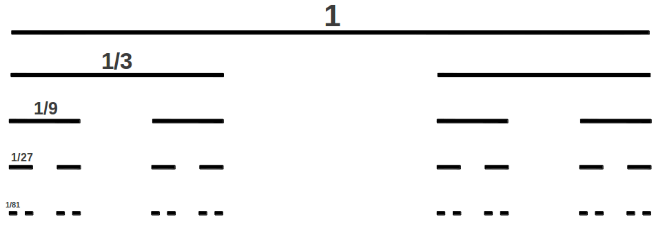
After two steps you have four intervals: [0,1/9], [2/9,1/3], [2/3, 7/9], and [8/9,1]. After three steps you have eight intervals of length 1/27. After k steps you have 2^k intervals of length 3^-k.

The Cantor set is the set of all points that never get removed during this infinite process. The Cantor set clearly contains infinitely many points because it contains the endpoints of the intervals that are removed: 0, 1, 1/3, 2/3, 1/9. 2/9, 7/9, 8/9, and so forth. Less intuitive is the fact that the cardinality of the Cantor set is uncountably infinite even though it is a set of measure zero.

Construction of the Cantor function

The Cantor function F: [0,1] → [0,1] can be defined iteratively in a way that reflects the construction of the Cantor middle-thirds set. The function is shown at the top of this article.

• At step 0, define the function on the endpoints of the [0,1] interval by F(0)=0 and F(1)=1.
• At step 1, define the function on the closed interval [1/3, 2/3] to be 1/2.
• At step 2, define the function on [1/9, 2/9] to be 1/4. Define the function on [7/9, 8/9] to be 3/4.
• Continue this construction. At each step, the function is defined on the closure of the middle-thirds intervals so that the function value is halfway between adjacent values. The function looks like a staircase with steps of difference heights and widths. The function is constant on every middle-thirds interval, but nevertheless is continuous and monotonically nondecreasing.

Visualizing the Cantor function in SAS

This is a SAS-related blog, so I want to visualize the Cantor function in SAS. The middle-third intervals during the kth step of the construction have length 3^-k, so you can stop the construction after a small number of iterations and get a decent approximation. I'll use k=8 steps.

Although the Cantor set and function were defined geometrically, they have an equivalent definition in terms of decimal expansion. The Cantor set is the set of decimal values that can be written in base 3 without using the '1' digit. In other words, elements of the Cantor set have the form x = 0.a₁a₂a₃... (base 3), where a_i equals 0 or 2.

An equivalent definition in terms of fractions is x = Σ_i a_i3^-i where a_i equals 0 or 2. Although the sum is infinite, you can approximate the Cantor set by truncating the series after finitely many terms. A sum like this can be expressed as an inner product x = a*v` where a is a k-element row vector that contains 0s and 2s and v is a vector that contains the elements {1/3, 1/9, 1/27, ..., 1/3^-k}.

You can define B to be a matrix with k columns and 2^k rows that contains all combinations of 0s and 2s. Then the matrix product B*v is an approximation to the Cantor set after k steps of the construction. It contains the right-hand endpoints of the middle-third intervals.

In SAS/IML you can use the EXPANDGRID function to create a matrix whose rows contain all combinations of 0s and 2s. The ## operator raises an element to a power. Therefore the following statements construct and visualize the Cantor function. With a little more effort, you can write a few more statements that improve the approximation and add fractional tick marks to the axes, as shown in the graph at the top of this article.

proc iml;
/* rows of B contain all 8-digit combinations of 0s and 2s */ 
B = expandgrid({0 2}, {0 2}, {0 2}, {0 2}, {0 2}, {0 2}, {0 2}, {0 2});
B = B[2:nrow(B),];      /* remove first row of zeros */
k = ncol(B);            /* k = 8 */
 
v = 3##(-(1:k));       /* vector of powers 3^{-i} */
t = B * v`;            /* x values: right-hand endpts of middle-third intervals */
 
u = 2##(-(1:k));       /* vector of powers 2^{-i} */
f = B/2 * u`;          /* y values: Cantor function on Cantor set */
call series(t, f);     /* graph the Cantor function */

I think this is a very cool construction. Although the Cantor function is defined iteratively, there are no loops in this program. The loops are replaced by matrix multiplication and vectors. The power of a matrix language is that it enables you to compute complex quantities with only a few lines of programming.

Do you have a favorite example from math or statistics that changed the way that you look at the world? Leave a comment.

References

This short article cannot discuss all the mathematically interesting features of the Cantor set and Cantor function. The following references are provided for the readers who want additional information:

• Construction of the Cantor set and Cantor function.
• MathWorld article on the Cantor function, with references to mathematical articles.