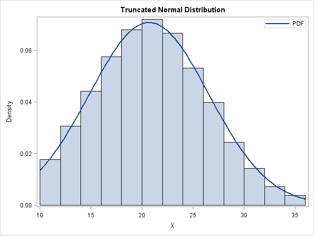
The truncated normal distribution TN(μ, σ, a, b) is the distribution of a normal random variable with mean μ and standard deviation σ that is truncated on the interval [a, b]. I previously blogged about how to implement the truncated normal distribution in SAS.
A friend wanted to simulate data from this distribution on the interval [10, 36], but did not have values of μ and σ. Instead, he needed the mean and standard deviation of the TN distribution to be 21.1 and 5.3 to match some published results. How can you find the (μ, σ) values that produce the specified moments?
This is an example of an "inverse problem." Let λ be the mean of the TN(μ, σ, 10, 36) distribution. Let δ be the standard deviation. Given target values λ* and δ*, what values of μ and σ produce a distribution TN(μ, σ, a, b) that has mean λ* and standard deviation δ*?
If λ and δ have simple expressions in terms of μ and σ, you might be able to analytically solve the two equations in two unknowns, but in general the equations will not have a closed-form solution. However, you can solve the problem numerically. The following SAS/IML program uses the formulas from the Wikipedia article on the truncated normal distribution to define a function that returns the mean and standard deviation of the TN distribution:
proc iml;
start TNMoments(mu, sigma, a, b);
   alpha = (a-mu)/sigma;
   beta = (b-mu)/sigma;
   Z = CDF("Normal", beta) - CDF("Normal", alpha);
   phi_a = PDF("Normal", alpha);
   phi_b = PDF("Normal", beta);
   /* express mean and std dev of TN distribution in terms of mu and sigma */
   lambda = mu + (phi_a - phi_b)/Z # sigma;    /* mean of TN distribution */
   s = 1 + (alpha#phi_a - beta#phi_b)/Z - ((phi_a - phi_b)/Z)##2;
   delta = sigma # sqrt(s);                    /* std dev of TN distribution */
   return( lambda || delta );
finish; |
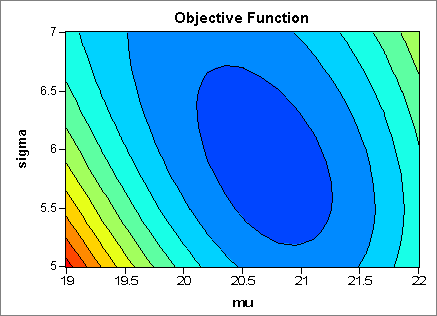
How does the mean and standard deviation of the TN distribution depend on the μ and σ parameters? Let S(μ, σ) be the function (defined above) that returns the vector of moments (λ, δ) for the TN distribution with parameters (μ, σ). Define the objective function G(μ, σ) = S(μ, σ) - (λ*, δ*). The following contour plot of || G ||2 shows that the desired parameters are somewhere in the dark blue region.
Either of the following will find zeros of G:
- Solve for a root of G. I've previously blogged about how to use a root-finding algorithm such as Newton's method.
- Solve for the value of (μ, σ) that minimizes || G(μ, σ) ||2. The SAS/IML language provides several algorithms for optimizing functions, including the NLPNRA subroutine, which is used for the subsequent analysis.
Because I've previously blogged on root-finding, I'll choose the optimization method for this article. The following statements define the function to minimize. The values (μ, σ) = (21, 6) are used to provide the optimization routine with an initial guess for the optimal value.
targetMean = 21.1;  targetSD = 5.3;   /* global vars used in the optimization */
a = 10; b = 36;

start SSQObjective(param) global(targetMean, targetSD, a, b);
   mu = param[,1]; sigma = param[,2];
   G = TNMoments(mu, sigma, a, b) - (targetMean || targetSD);
   return( G[,##] );           /* return sum of squares of elements = || G ||^2 */
finish;

x0 = {21 6};                   /* initial guess */
call nlpnra(rc, soln, "SSQObjective", x0);
print soln[c={"mu" "sigma"}]; |
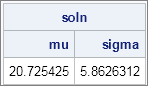
The optimization routine gives (μ, σ) = (20.7, 5.86) as the parameter values that correspond to a distribution with the specified mean and standard deviation. The histogram at the top of this article shows a random draw from the TN(20.7, 5.86, 10, 36) distribution, along with an overlay of the corresponding PDF. The mean and standard deviation of the sample are close to the target values (21.1 and 5.3, respectively).
Even if you never have a need for the truncated normal distribution, this article shows a useful technique: how to choose parameter values for a distribution so that the distribution has certain properties. In this case, the properties are the mean and standard deviation, but you can specify any two independent quantities and obtain similar results. The key is to express the target quantities in terms of the parameters, and use root-finding or optimization techniques to obtain the desired parameter values.
