It is easy to use the SGPLOT procedure in SAS to plot the graph of a well-behaved continuous function: just create a data set of the (x,y) values on some domain and use the SERIES statement to connect the points. However, to plot the graph of a discontinuous function correctly requires more thought.

In statistics, discontinuous functions arise with moderate frequency. Empirical cumulative distribution functions are discontinuous, as are many bounded probability density functions. A simple example is the (continuous) uniform density function, which is defined as 1 on the interval [0, 1], and 0 outside of that interval.

If you want to graph the standard uniform density function, you might attempt the following:

data UniformPDF_Orig;
do x = -1 to 2 by 0.05;
   y = (x>=0 & x<=1);
   output;
end;
run;
 
title "Discontinuous Function: First Attempt";
proc sgplot data=UniformPDF_Orig;
   series x=x y=y;
   refline 0 1 / axis=x lineattrs=(pattern=dash);
   yaxis min=-0.1 max=1.1;
run;

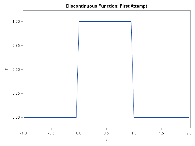
Although the graph shows the basic idea of the uniform density, it is not accurate because the SERIES statement just "connects the dots," and so the graph displays a line segment with a large slope on the interval [–0.05, 0], and a line segment with a large negative slope on the interval [0.95, 1]. If you reduce the interval between consecutive points (for example, by using 0.01 as the step size in the DO loop), you can reduce the visual impact of the error, but it is still there.

If you know the points of discontinuity, then you can make a better graph by generating points on intervals for which the function is continuous. You can enumerate each interval and then use the GROUP= option on the SERIES statement to plot the graph on each interval, as follows:

data UniformPDF;
domain = 1;
do x = -1 to 0 by 0.05;
   y = 0; output;
end;
domain = 2;
do x = 0 to 1 by 0.05;
   y = 1; output;
end;
domain = 3;
do x = 1 to 2 by 0.05;
   y = 0; output;
end;
run;
 
title "Discontinuous Function: Better Version";
proc sgplot data=UniformPDF noautolegend;
   series x=x y=y / group=domain lineattrs=GraphFit;
   refline 0 1 / axis=x lineattrs=(pattern=dash);
   yaxis min=-0.1 max=1.1;
run;

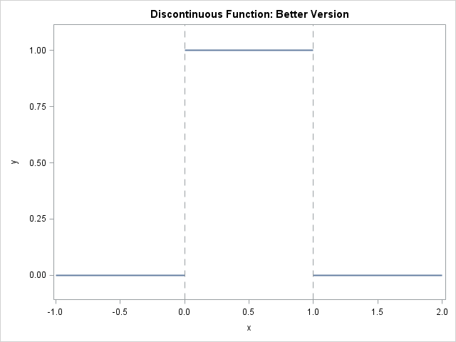
The GROUP= option tells the SGPLOT procedure to plot three distinct curves, and not to connect them. The resulting graph is more accurate.

Thanks to Warren Kuhfeld for suggesting this topic.