Last week I wrote about how to compute sample quantiles and weighted quantiles in SAS. As part of that article, I needed to draw some step functions. Recall that a step function is a piecewise constant function that jumps by a certain amount at a finite number of points.

Graph an empirical CDF

In statistics, the canonical step function is the empirical cumulative distribution function. Given a set of data values x₁ ≤ x₂ ≤ ... ≤ x_n the empirical distribution function (ECDF) is the step function defined by
     F(t) = (number of data values ≤ t) / n.
Notice that an ECDF is constant on each half-open interval [x_i, x_i+1).

The easiest way to visualize the ECDF in SAS is to use the CDFPLOT statement in PROC UNIVARIATE. The following DATA step creates a set of nine observations. Two values are repeated. The call to PROC UNIVARIATE creates a graph of the empirical CDF:

data A;
input x @@;
datalines;
3.7  1.0  2.2  4.1  5.0  1.9  3.0  2.2  4.1
;
 
ods select cdfplot;
proc univariate data=A;
cdfplot x / vscale=proportion 
         odstitle="Empirical CDF" odstitle2="PROC UNIVARIATE";
ods output cdfplot=outCDF;   /* data set contains ECDF values */
run;

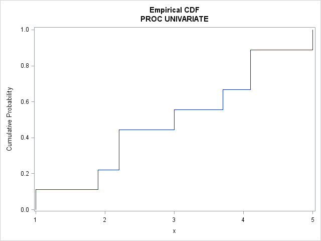
The ECDF jumps by 1/n = 1/9 at each sorted data value. Because the values 2.2 and 4.1 appear twice in the data, the ECDF jumps by 2/9 at those data values. The ECDF is 0 for any point less than the minimum data value; it is 1 for any point greater than or equal to the maximum data value.

Create an ECDF graph manually

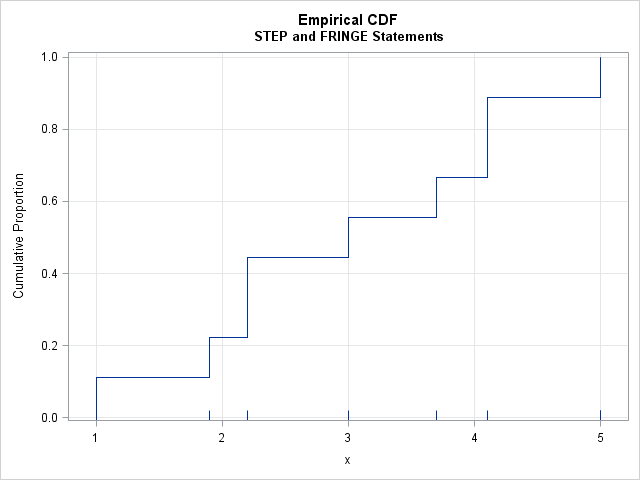
In the previous call to PROC UNIVARIATE, the ODS OUTPUT statement writes a SAS data set that contains the data values in sorted order and the value of the ECDF at each data value. You can use this output data set and the STEP statement in PROC SGPLOT to create your own graph of the ECDF. This gives you complete control over colors, labels, background grids, and other graphical attributes. You can also overlay other plots on the ECDF. For example, the following call to PROC SGPLOT creates an ECDF, adds a background grid, and overlays a fringe plot that shows individual data values:

title "Empirical CDF";
title2 "STEP and FRINGE Statements";
proc sgplot data=outCDF noautolegend;
   step x=ECDFX y=ECDFY;          /* variable names created by PROC UNIVARIATE */
   fringe ECDFX;
   xaxis grid label="x" offsetmin=0.05 offsetmax=0.05;
   yaxis grid min=0 label="Cumulative Proportion";
run;

Graph an arbitrary step function in SAS

For the ECDF, we used PROC UNIVARIATE to create a data set that contains the (X,Y) coordinates of each "corner" in the plot. For a general discontinuous function, you need to create a similar data set manually. If you can create the data set, you can use the STEP statement to visualize an arbitrary piecewise constant function.

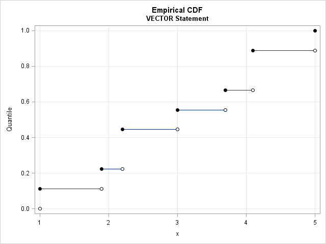
Some users might want to omit the vertical lines in the graph in order to emphasize the discontinuous nature of the function. For example, the adjacent graph is an alternative approach to visualizing the ECDF. This graph emphasizes that the function is constant on intervals that are closed on the left and open on the right.

You can use the VECTOR statement in PROC SGPLOT to generate this graph. The VECTOR statement draws a line between two arbitrary points. The output from PROC UNIVARIATE provides the X and Y values for the plot, but you need to modify the data slightly because the VECTOR statement needs four variables: the starting and ending coordinates of each line segment.

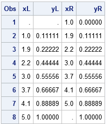
The adjacent table shows the shape of the data that is suitable for graphing with the VECTOR statement. You can see that the LAG function is useful for generating the xL column from the xR column. The yL and yR columns are identical except for the first observation because the ECDF is piecewise constant. The VECTOR statement connects the points (x_L, y_L) and (x_R, y_R), where the "L" subscript refers to left-hand endpoints and the "R" subscript refers to right-hand endpoints.

/* CDF is step function. 
   Each interval [x_i, x_{i+1}) is closed on the left and open on the right */
title "Empirical CDF";
title2 "VECTOR Statement";
proc sgplot data=ECDF noautolegend;
   vector x=xR y=yR / xorigin=xL yorigin=yL noarrowheads;
   scatter x=xL y=yL / markerattrs=(symbol=CircleFilled color=black);      /* closed */
   scatter x=xR y=yR / filledoutlinedmarkers markerfillattrs=(color=white) /* open */
                       markerattrs=(symbol=CircleFilled color=black);
   xaxis grid label="x";
   yaxis grid min=0 max=1 label="Quantile";
run;

In conclusion, there are several ways to visualize an empirical CDF in SAS. You can also visualize the graph of a general piecewise constant function. You can choose either the STEP statement or the VECTOR statement in PROC SGPLOT to visualize the graph.